Multi-cost prioritization with prioritizr SyncroSim
This tutorial provides an overview of working with prioritizr in SyncroSim Studio to demonstrate how to integrate multiple cost-layers into a lake conservation problem. A special thank you to Jeffrey Hanson for extensive and detailed support with the multi-cost methodology. This tutorial covers the following steps:
Step 1. Creating a prioritizr SyncroSim library
In SyncroSim, a library is a file with extension .ssim that stores all the model’s inputs and outputs in a format specific to a given package. To load the pre-configured library:
1. Open SyncroSim Studio.
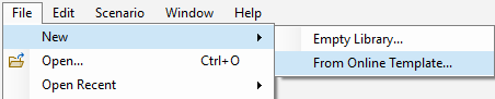
2. Select File > New > From Online Template….
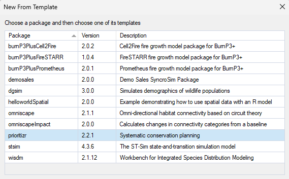
b. From the list of template libraries, select the Multi-Cost Prioritization (Ontario, Canada) template library.
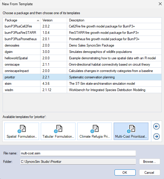
c. If desired, you may edit the File name, and change the Folder by clicking on the Browse button.
d. When done, click OK.
A new library has been created based on the selected template, and SyncroSim will have automatically opened and displayed it in the Explorer window.
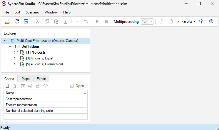
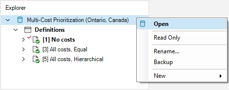
3. Double-click on the library name, Multi-Cost Prioritization (Ontario, Canada), to open the library properties window. You may also right-click on the library name and select Open from the context menu.
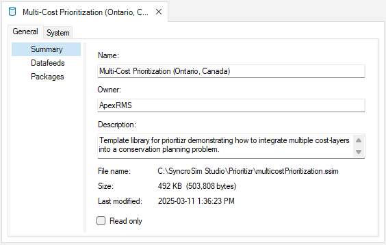
4. The Summary datasheet contains the metadata for the library.
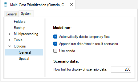
5. Next, navigate to the Systems tab, Options node, General datasheet, and make sure Use conda is disabled.
6. Close the library properties window.
Next, you will review the target feature data for the conservation prioritization problem.
7. From the Explorer window, right-click on Definitions and select Open from the context menu.
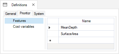
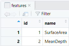
8. Under the Prioritizr tab, select the Features datasheet, which lists the variables that will be taken into account in the prioritization process. Here, the feature data corresponds to two lake property variables: MeanDepth and SurfaceArea. This datasheet was automatically populated once the first scenario was run.
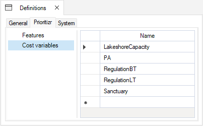
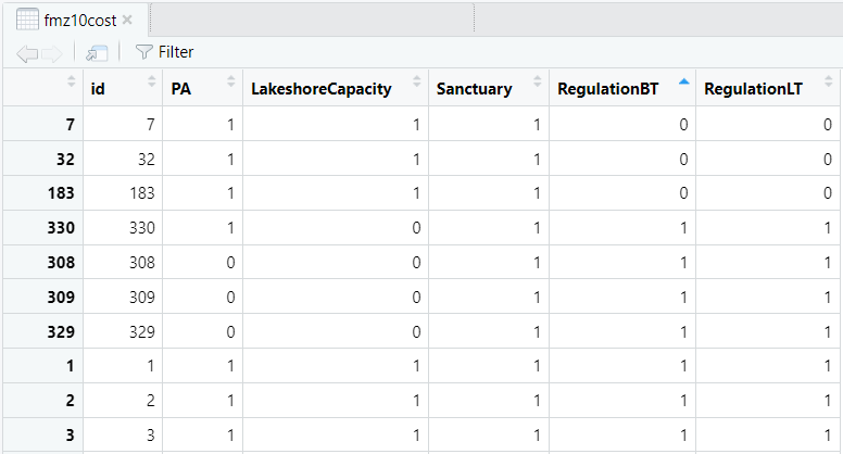
9. Next, open the Cost variables datasheet, which lists the cost variables that will be taken into account in the prioritization process. Here, all are binary variables that represent whether a lake (i.e., planning unit) has a protection cost (1) or not (0). This datasheet was also automatically populated, but once the first multi-cost prioritization scenario was run.
Now you will review the inputs for the No costs scenario, which provides a baseline where no costs are considered in the prioritization. This scenario is required, as it provides a baseline from which the multi-cost optimization builds. In SyncroSim, each scenario contains the model inputs associated with a model run.
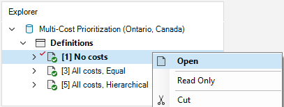
10. In the Explorer window, select the pre-configured scenario No costs and double-click it to open its properties. You may also right-click on the scenario name and select Open from the context menu.
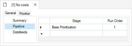
11. Navigate to the Pipeline datasheet. Pipeline stages call on a transformer (i.e., script) which takes the inputs from SyncroSim, runs a model, and returns the results to SyncroSim. Under the Stage column, note that a single pipeline stage is set, called Base Prioritization.
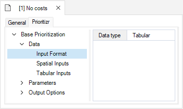
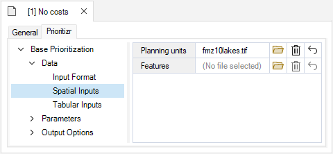
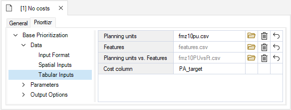
12. Navigate to the Prioritizr tab and expand the Base Prioritization > Data nodes.
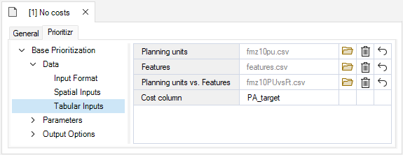
ii. Features – a data table listing the feature variables. These are listed under the column name, with an associated ID.
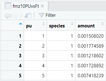
iii. Planning units vs. Features – a data table listing for each lake (under the pu column), the value (under the amount column) associated with each feature variable (under the species column).
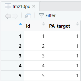
iv. Cost column – corresponds to the column in the Planning units input representing the cost variable.
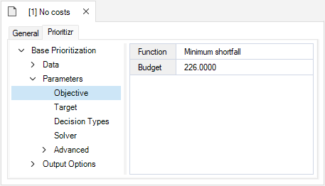
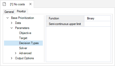
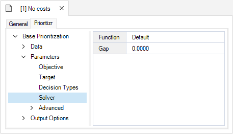
13. Expand the Parameters node.
ii. Budget – this number represents the maximum allowed cost of the prioritization. Here, the budgets is used to ensure that 30% of lakes in the study area are represented in the solution, which corresponds to 226.
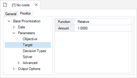
ii. Amount – specifies the desired level of feature representation in the study area. In this example, it is set to 1.0, so that each feature would ideally have 100% of its distribution covered by the prioritization.
ii. Gap – represents the gap to optimality and is set to a value of 0. This gap is relative and expresses the acceptable deviance from the optimal objective. In this example, a value of 0 will result in the solver only stopping when it has found the best possible solution.
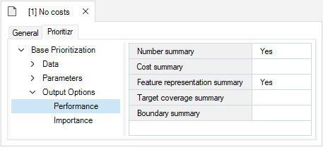
14. Expand the Output Options node and open the Performance datasheet to review the following inputs set to Yes:
ii. Feature representation summary – calculates how well features are represented by the solution to the conservation planning problem.
Step 2. Visualizing and comparing results across scenarios
The Multi-Cost Prioritization (Ontario, Canada) template library already contains the results for each scenario. Before exploring additional scenarios, you will view the main results for the No costs scenario.
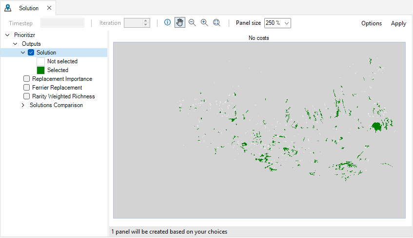
1. Navigate to the Maps tab, and double click on the pre-configured Solution map. The Solution map shows which planning units have been selected for prioritization given the input data and parameters.
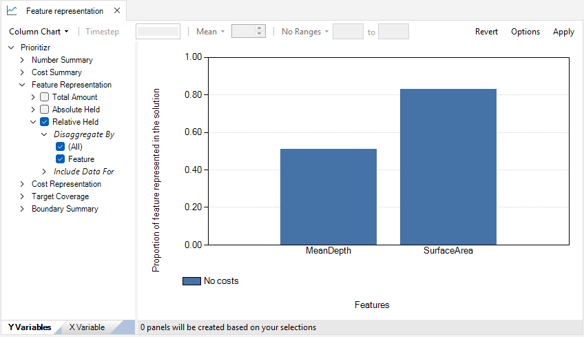
2. Navigate to the Charts tab, and double click on the pre-configured Feature representation chart. The Feature representation chart shows the proportion of mean depth and surface area represented in the No costs scenario solution. For instance, 51% of all the lakes’ mean depth and 83% of all the lakes’ surface area was represented in the solution.
3. Close the chart results panel.
Now, you will review the additional scenarios and explore how they differ from the No costs solution, which are built as a dependency of the No costs scenario.
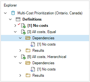
4. In the Explorer window, expand the All costs, Equal > Dependencies and All costs, Hierarchical > Dependencies nodes to reveal the No costs scenario dependency.
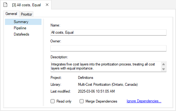
5. Select the pre-configured scenario All costs, Equal and double-click it to open its properties. You may also right-click on the scenario name and select Open from the context menu.
6. In the Summary datasheet, note the Description that says that this scenario “integrates five cost layers into the prioritization process, treating all cost layers with equal importance”.
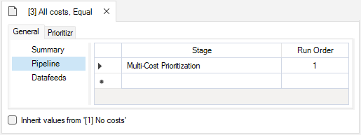
7. Open the Pipeline datasheet and note that the “Inherit values from ‘[1] No costs’” checkbox in the bottom left corner is not marked, and new pipeline stage is set, called Multi-Cost Prioritization.
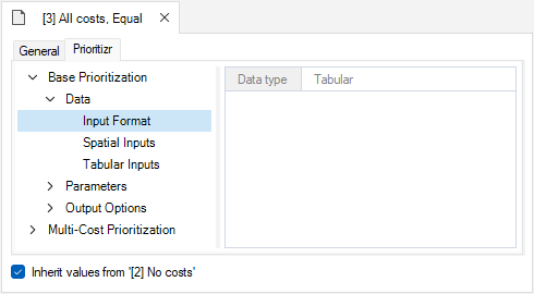
8. Navigate to the Prioritizr tab, expand the Base Prioritization > Data nodes, and open the Input Format datasheet. Notice that this information cannot be edited (i.e., greyed out) and the “Inherit values from ‘[2] No costs’” checkbox in the bottom left corner is marked. This indicates that values within this datasheet and others are derived from the No costs result scenario acting as a dependency.
9. Expand the Multi-Cost Prioritization node and open the Data datasheet to review the following input:
10. Next, open the Parameters datasheet and review the following inputs:
ii. Initial optimality gap – set to 0.9. Used to calculate the target for the cost-optimized solution, based on how well the objective was achieved in the baseline solution. Values closer to 1 result in solutions that tend to sacrifice feature representation for less costly solutions.
iii. Cost optimality gap – Default value was automatically populated, but parameter is not relevant for the equal cost-optimization method.
iv. Budget increments – Default value was automatically populated, but parameter is not relevant for the equal cost-optimization method.
v. Budget padding – Default value was automatically populated, but parameter is not relevant for the equal cost-optimization method.
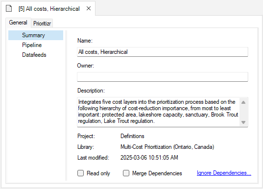
11. Select the pre-configured scenario All costs, Hierarchical and double-click it to open its properties. You may also right-click on the scenario name and select Open from the context menu.
12. In the Summary datasheet, note the Description that says that this scenario “integrates five cost layers into the prioritization process based on the following hierarchy of cost-reduction importance, from most to least important: protected area, lakeshore capacity, sanctuary, Brook Trout regulation, Lake Trout regulation”.
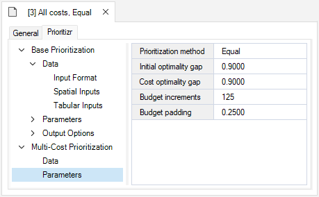
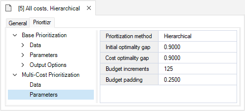
13. Navigate to the Prioritizr tab, expand the Multi-Cost Prioritization node, open the Parameters datasheet and review the following inputs:
ii. Initial optimality gap – set to 0.9. Used to calculate the target for the cost-optimized solution, based on how well the objective was achieved in the baseline solution. Values closer to 1 result in solutions that tend to sacrifice feature representation for less costly solutions.
iii. Cost optimality gap – set to 0.9. Used to calculate a constraint on the cost of the cost-optimized solution, according to the previously optimized cost layers. Values closer to 1 result in accepting greater differences in costs between layers.
iv. Budget increments – set to 125. Defines the length of the vector of budget increments, which are used to iteratively find the budget under which a feasible solution can be found, while ensuring the solution does not cost "too much". Higher values will take longer to run, but may be able to find a slightly more cost effective solution.
v. Budget padding – set to 0.25. For each cost variable, it is used to calculate the budget increment values, based on the cost of the solution with only the target cost variable. Represents a percentage increase in cost. Higher values will results in a larger range of budgets being attempted.
14. Close the scenario properties.
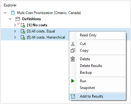
15. In the Explorer window, hold Shift and click on both the All costs, Equal and All costs, Hierarchical scenarios to select them. Right-click and select Add to Results from the context menu to simultaneously add each scenario to the results.
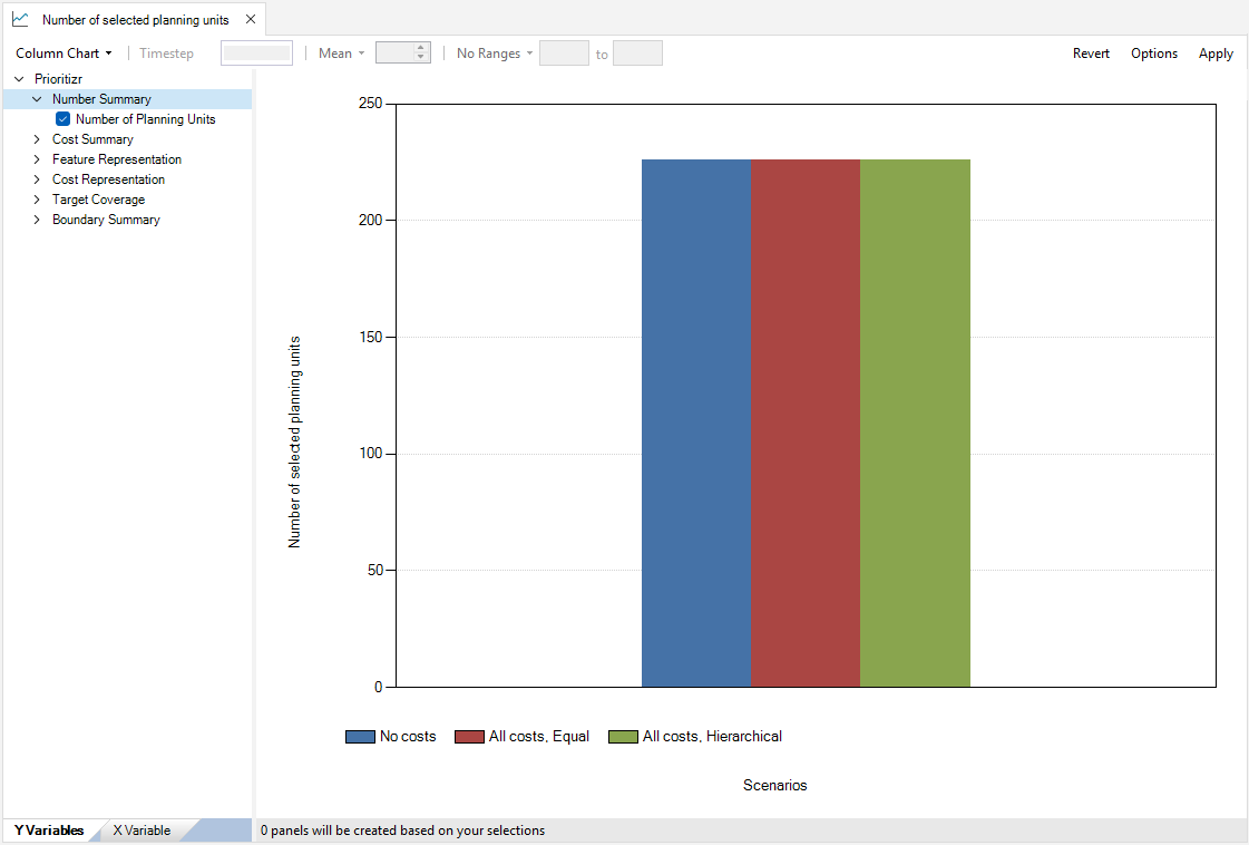
16. Navigate to the Charts tab, and double-click on the pre-configured Number of selected planning units chart. This chart displays the total number of planning units in the solution per scenario. In this example, 226 lakes were selected in the solution, showing the budget was met in all scenarios.
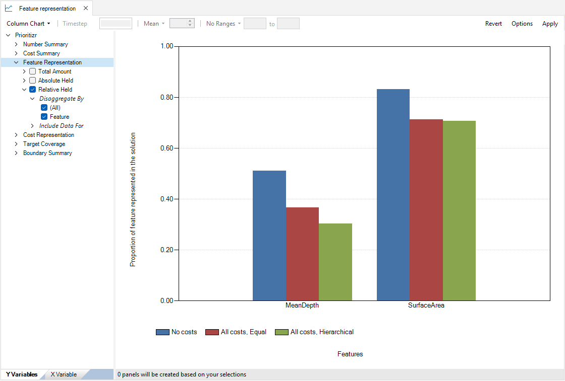
21. Next, double-click on the pre-configured Feature representation chart. This chart displays the proportion of each feature (i.e., mean lake depth and lake surface area) represented in the solution for each scenario. Note that the cost-optimized scenarios resulted in less feature representation, suggesting an intuitive trade-off between cost restrictions and feature representation.
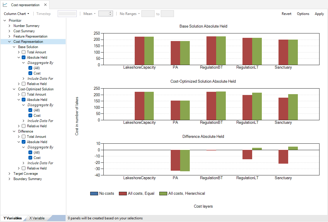
16. Next, double-click on the pre-configured Cost representation chart. Across all charts, the x-axis represents the five different cost variables and the y-axis represents the solution cost in terms of number of lakes.
ii. The middle chart, Cost-Optimized Solution Absolute Held, shows the cost represented in the cost-optimized solutions for each cost variable. For instance, given the lakes selected in the solution to the All costs, Equal scenario, 200 lakes show a RegulationLT cost. The cost is slightly higher under the All costs, Hierarchical scenario.
iii. The bottom chart, Difference Absolute Held, shows the amount of change between the baseline and each cost-optimized scenario. Here, negative values represent a reduction in cost in the cost-optimized solution, and positive values represent an increase in cost. For example, there was a reduction in PA costs of over 30 lakes in both scenarios. In turn, whereas RegulationLT cost decreased under the All costs, Equal scenario, it increased under the All costs, Hierarchical scenario. That is because the Hierarchical method prioritized reducing cost in the most important layer (PA) at the detriment of others.
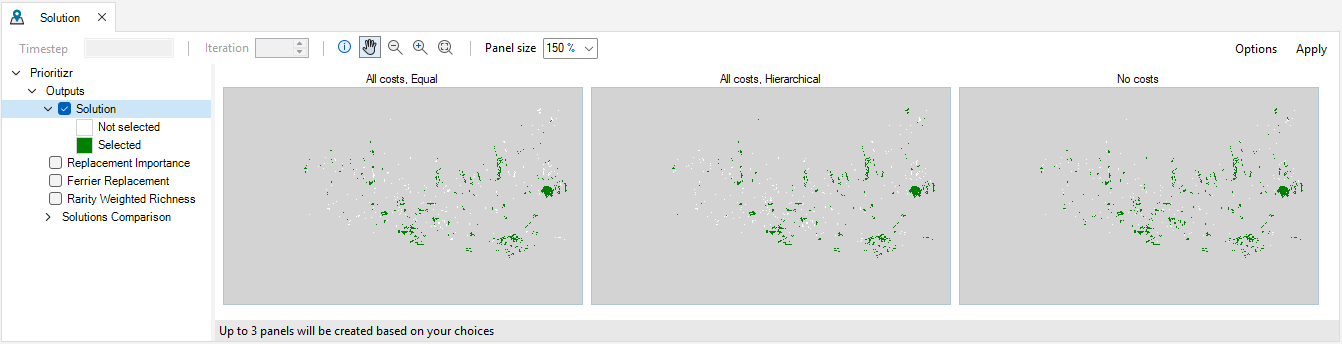
23. Now, navigate to the Maps tab, and double-click on the pre-configured Solution map. This map displays the lakes that were selected in the solution under each scenario. The package, however, offers a better way to compare the results.
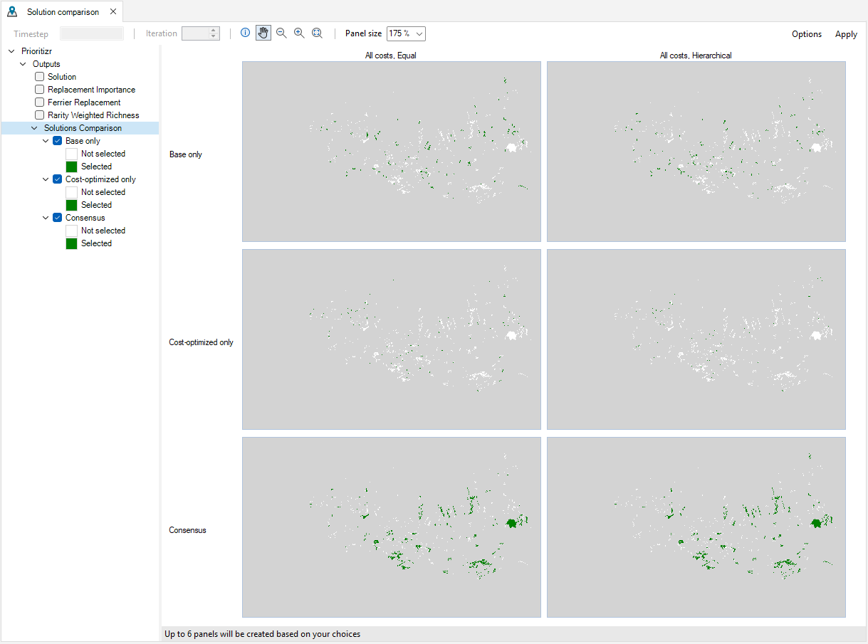
24. Double-click on the pre-configured Solution comparison map. This map is only computed by the Multi-Cost Prioritization stage scenarios, so the No costs scenario was removed from results. The Base only maps display which lakes were only selected under the baseline scenario (No cost). The Cost-optimized only maps show which lakes were only selected when the solution was optimized for cost, under the equal or hierarchical prioritization methods. The Consensus maps display which lakes were selected in both the baseline and cost-optimized solutions.
This tutorial demonstrated how prioritizr can be used to build tabular formulations of conservation problems, with a spatial visualization of the results, and covered how to account for multiple cost layers in the prioritization process. To explore more with prioritizr, see the tutorials page.