Spatial conservation prioritization with prioritizr SyncroSim
This tutorial provides an overview of working with prioritizr in SyncroSim Studio to create and solve a spatial conservation problem. Here, you will review a pre-configured library that reproduces the example available in the prioritizr R package documentation. It covers the following steps:
Step 1. Creating a prioritizr SyncroSim library
In SyncroSim, a library is a file with extension .ssim that stores all the model’s inputs and outputs in a format specific to a given package. To load the pre-configured library:
1. Open SyncroSim Studio.
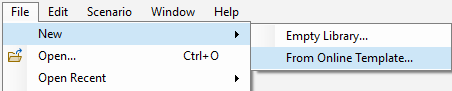
2. Select File > New > From Online Template….
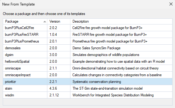
b. From the list of template libraries, select the Spatial Formulation Example.
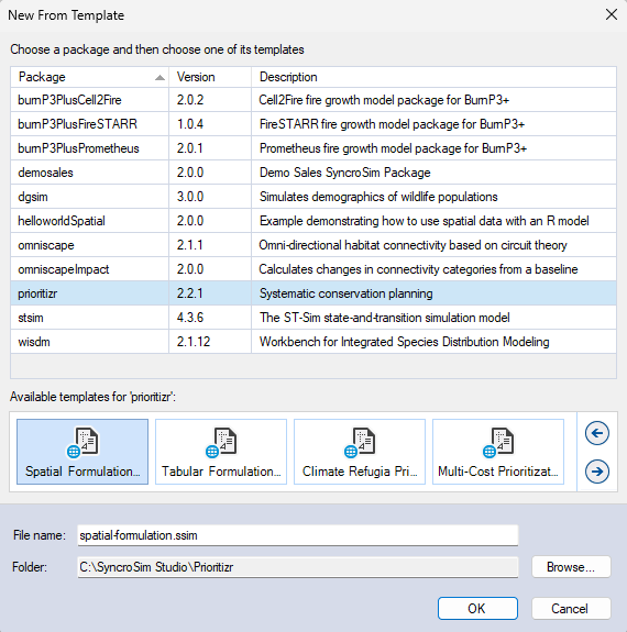
c. If desired, you may edit the File name, and change the Folder by clicking on the Browse button.
d. When done, click OK.
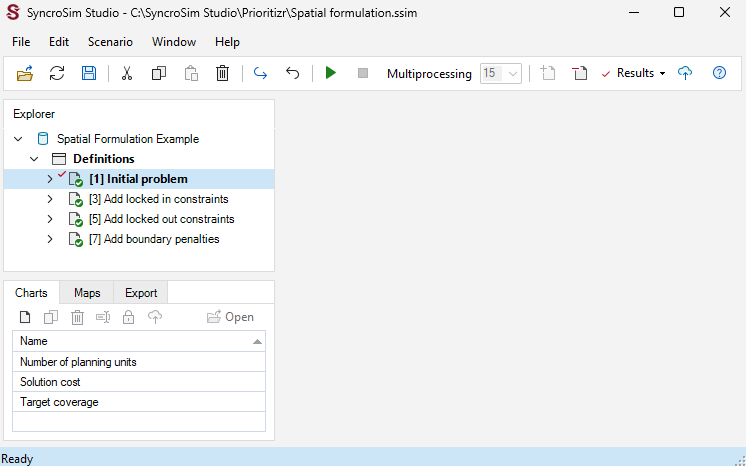
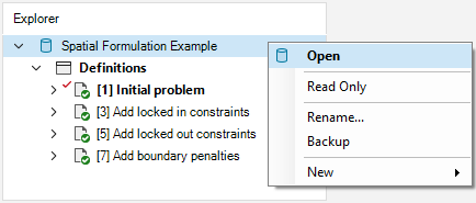
A new library has been created based on the selected template, and SyncroSim will have automatically opened and displayed it in the Explorer window.
3. Double-click on the library name, Spatial Formulation Example, to open the library properties window. You may also right-click on the library name and select Open from the context menu.
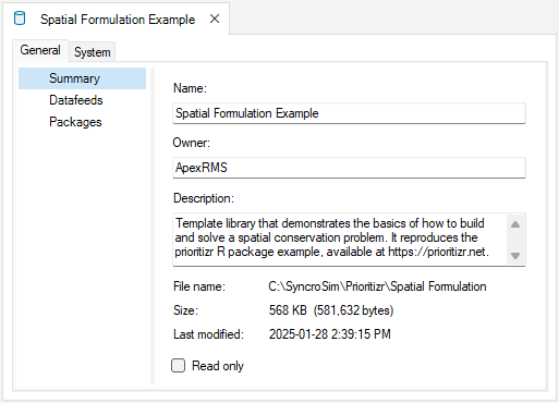
4. The Summary datasheet contains the metadata for the library.
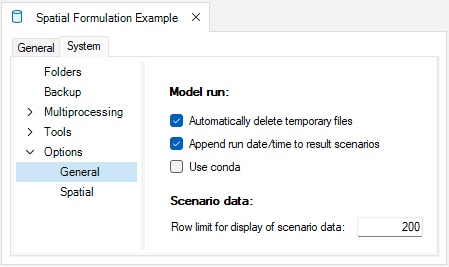
5. Next, navigate to the System tab, Options node, General datasheet, and make sure Use conda is disabled.
6. Close the library properties window.
Next, you will review the target feature data for the conservation prioritization problem.
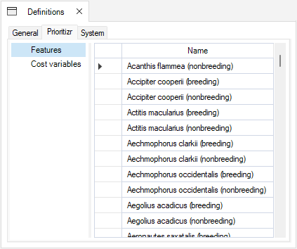
7. From the Explorer window, right-click on Definitions and select Open from the context menu.
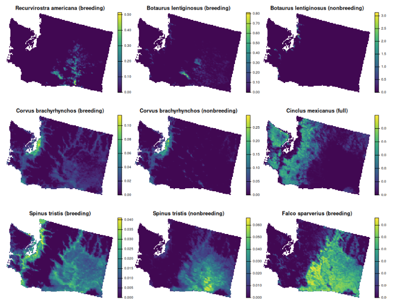
8. Under the Prioritizr tab, select the Features datasheet, which lists the variables that will be taken into account in the prioritization process. In this library, note that the feature data corresponds to different bird species. This datasheet was automatically populated once the first scenario was run.
Now, you will review the inputs for the Initial problem scenario, which sets up the initial problem formulation out of which the other scenarios are built. In SyncroSim, each scenario contains the model inputs associated with a model run.
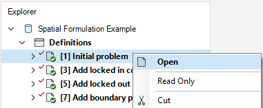
9. In the Explorer window, select the pre-configured scenario Initial problem and double-click it to open its properties. You may also right-click on the scenario name and select Open from the context menu.
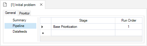
10. Navigate to the Pipeline datasheet. Pipeline stages call on a transformer (i.e., script) which takes the inputs from SyncroSim, runs a model, and returns the results to SyncroSim. Under the Stage column, note that a single pipeline stage is set, called Base Prioritization.
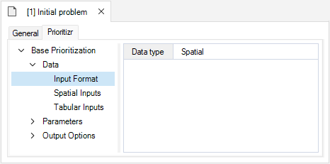
11. Navigate to the Prioritizr tab and expand the Base Prioritization > Data nodes.
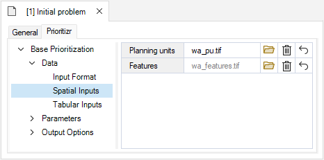
ii. Features – a multi-layer raster file of the conservation feature data (i.e., bird species). Layers describe the spatial distribution of each bird species, where cell values denote the relative abundance of individuals.
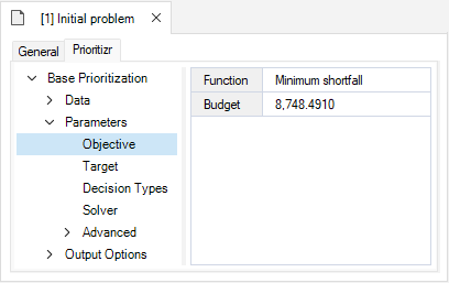
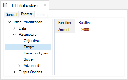
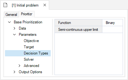
12. Expand the Parameters node.
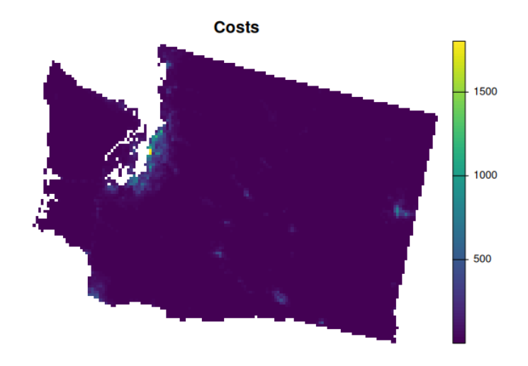
ii. Budget – this number represents the maximum allowed cost of the prioritization. Specifically, this value is set to $8,748.4910, which represents 5% of the total land value in the study area.
ii. Amount – specifies the desired level of feature representation in the study area. In this example, it is set to 0.2, so that each feature would ideally have 20% of its distribution covered by the prioritization.
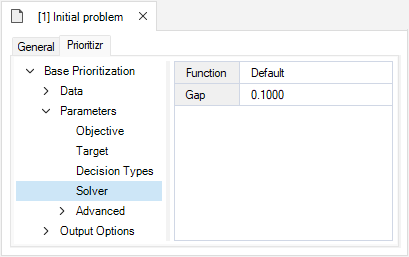
ii. Gap – represents the gap to optimality, and is set to a default value of 0.1. This gap is relative and expresses the acceptable deviance from the optimal objective. In this example, a value of 0.1 will result in the solver stopping when it has found a solution within 10% of optimality.
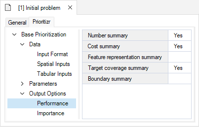
13. Expand the Output Options node and open the Performance datasheet to review the following inputs set to Yes:
ii. Cost summary – calculates the total cost of the solution to the conservation planning problem.
iii. Target coverage summary – calculates how well the feature representation targets are met by the solution to the conservation planning problem.
Step 2. Visualizing and comparing results across scenarios
The Spatial Formulation Example template library already contains the results for each scenario. Before exploring additional scenarios, you will view the main result for the Initial problem scenario.
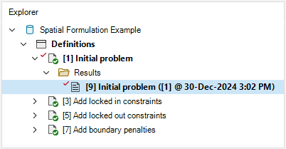
1. In the Explorer window, expand the Initial Problem > Results nodes to reveal the Inital Problem results scenario. This scenario contains the outputs of the model run, it is timestamped, and has a copy of all the input parameters.
2. Collapse the scenario node by clicking on the downward facing arrow beside the scenario name.
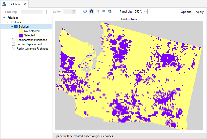
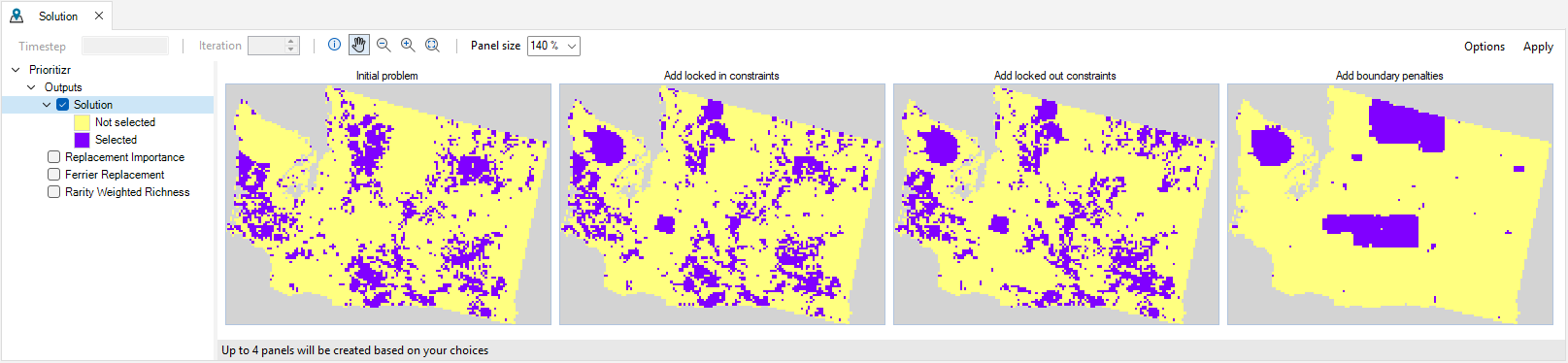
3. Navigate to the Maps tab, and double click on the pre-configured Solution map. The Solution map shows in purple which planning units have been selected for prioritization given the input data and parameters. Although this solution helps meet the representation targets, it does not account for existing protected areas inside the study area.
4. Close the results panels.
Now, you will review the additional scenarios and explore how they differ from the Initial problem.
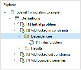
5. In the Explorer window, expand the Add locked in constraints > Dependencies nodes to reveal the Initial problem scenario dependency. This means that the Add locked in constraints scenario builds on the Initial problem scenario.
6. Select the pre-configured scenario Add locked in constraints and double-click it to open its properties. You may also right-click on the scenario name and select Open from the context menu.
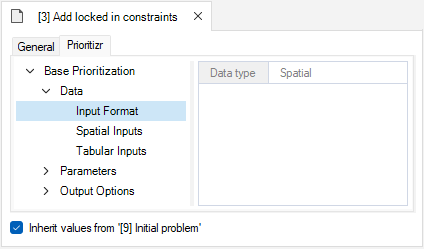
7. Navigate to the Prioritizr tab, expand the Base Prioritization > Data nodes, and open the Input Format datasheet. Notice that this information cannot be edited (i.e., greyed out) and the “Inherit values from ‘[9] Initial Problem’” checkbox in the bottom left corner is marked. This indicates that values within this datasheet and others are derived from the Initial Problem result scenario acting as a dependency.
8. Navigate to the Prioritizr tab, expand the Parameters > Advanced > Constraints nodes, and open the Locked In datasheet to review the following inputs:
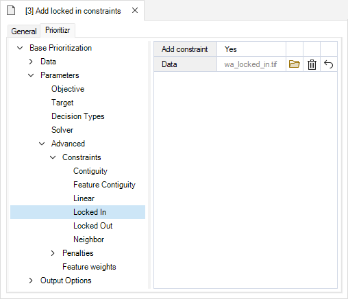
ii. Data – contains the spatial data (i.e., raster) specifying the locations of the areas to be locked in (e.g., protected areas).

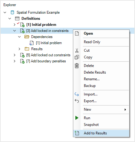
9. In the Explorer window, right-click on the Add locked in constraints scenario, and select Add to Results from the context menu.
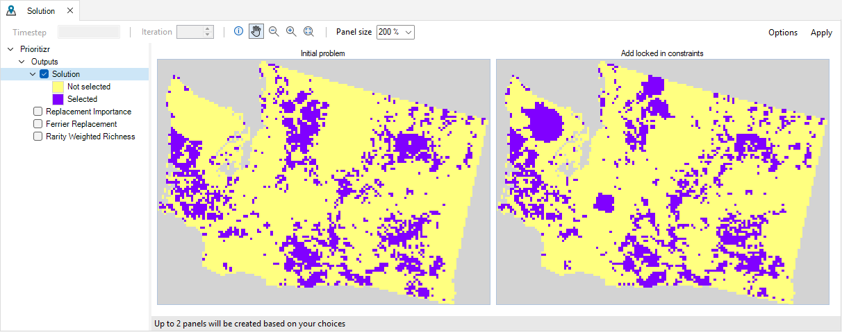
10. Navigate to the Maps tab and double click on the pre-configured Solution map. Notice that the Add locked in constrains results were added. This solution now accounts for existing protected areas inside the study area, resulting in an improved solution.
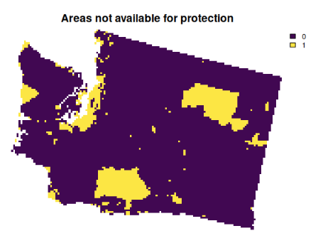
Yet, some places in the study area are not available for protection (e.g., due to land tenure). Consequently, the solution might not be practical for implementation. The Add locked out constraints scenario addresses this issue by constraining the pool of planning units that may be selected by the solution.
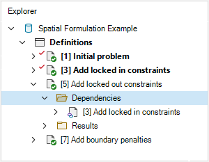
11. In the Explorer window, expand the Add locked out constraints > Dependencies nodes to reveal the Add locked in constraints scenario dependency. This means that this scenario builds on the previous scenario.
12. Select the pre-configured scenario Add locked out constraints and double-click it to open its properties. You may also right-click on the scenario name and select Open from the context menu.
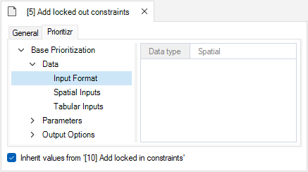
13. Navigate to the Prioritizr tab, expand the Base Prioritization > Data nodes, and open the Input Format datasheet. Notice that this information cannot be edited (i.e., greyed out) and the “Inherit values from ‘[10] Add locked in constraints’” checkbox in the bottom left corner is marked. This indicates that values within this datasheet and others are derived from the Add locked in constraints result scenario acting as a dependency.
14. Navigate to the Prioritizr tab, expand the Parameters > Advanced > Constraints nodes, and open the Locked Out datasheet to review the following inputs:
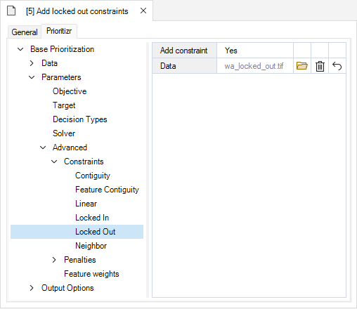
ii. Data – contains the spatial data (i.e., raster) specifying the locations of the areas to be locked out (e.g., areas not available for protection).
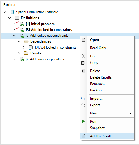
15. In the Explorer window, right-click on the Add locked out constraints scenario, and select Add to Results from the context menu.
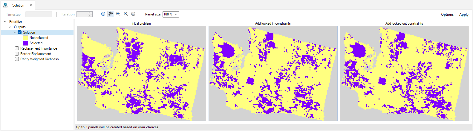
16. Navigate to the Maps tab, and double click on the pre-configured Solution map. Notice that the Add locked out constraints results were added. This solution now accounts for existing protected areas as well as areas that are not available for protection inside the study area, resulting in an even better solution.
However, the planning units selected from the solution are fairly fragmented. This can cause issues because fragmentation increases management costs and reduces conservation benefits through edge effects. The Add boundary penalties scenario addresses this final issue by adding penalties that punish overly fragmented solutions.
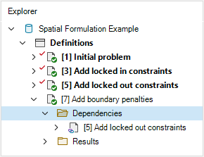
17. In the Explorer window, expand the Add boundary penalties > Dependencies nodes to reveal the Add locked out constraints scenario dependency. This means that this scenario builds on the previous scenario.
18. Select the pre-configured scenario Add boundary penalties and double-click it to open its properties. You may also right-click on the scenario name and select Open from the context menu.
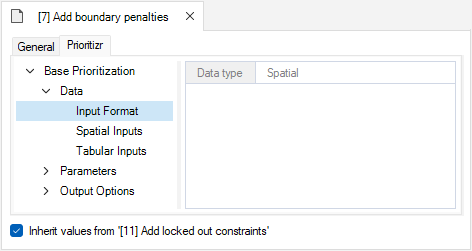
19. Navigate to the Prioritizr tab, expand the Base Prioritization > Data nodes, and open the Input Format datasheet. Notice that this information cannot be edited (i.e., greyed out) and the “Inherit values from ‘[11] Add locked in constraints’” checkbox in the bottom left corner is marked. This indicates that values within this datasheet and others are derived from the Add locked out constraints result scenario acting as a dependency.
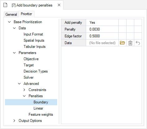
20. Navigate to the Prioritizr tab, expand the Parameters > Advanced > Penalties nodes, and open the Boundary datasheet to review the following inputs:
ii. Penalty – a value used to scale the importance of selecting planning units that are spatially clumped together compared to the main problem objective. Higher penalty values prefer solutions with a higher degree of spatial clumping, whereas smaller penalty values prefer solutions that are more spread out. In this example, the penalty is set to 0.003.
iii. Edge factor – a value used to specify the proportion to scale planning unit edges (borders) that do not have any neighboring planning units. In this example, the edge factor is set to 0.5.
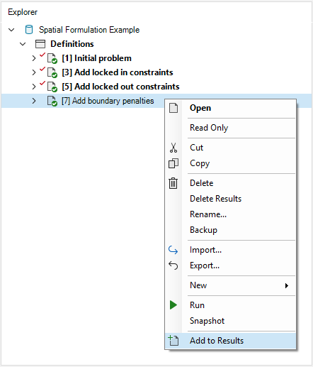
21. In the Explorer window, right-click on the Add boundary penalties scenario, and select Add to Results from the context menu.
22. Navigate to the Maps tab, and double click on the pre-configured Solution map. Notice that the Add boundary penalties results were added. This solution now accounts for protected areas, areas not available for protection, as well as highly fragmented areas inside the study area.
In addition to spatial representation of the solution, prioritizr also produces tabular summaries.
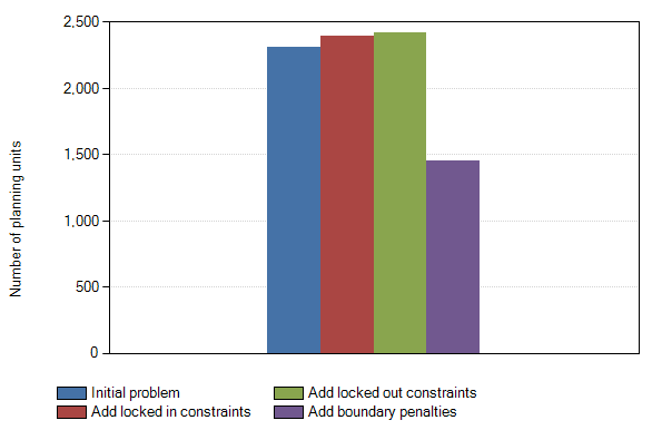
23. Navigate to the Charts tab and double-click on the pre-configured Number of planning units chart. Note that the number of planning units increases (i.e., fragmentation), until the boundary penalty was added.
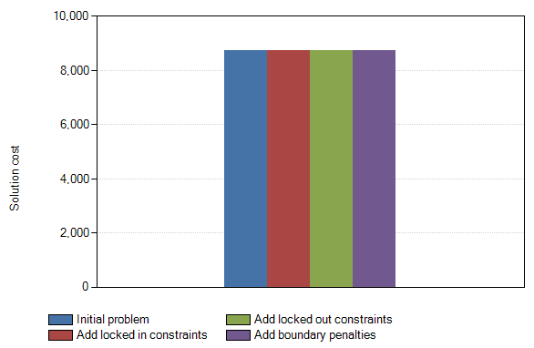
24. Next, double-click on the pre-configured Solution cost chart. Here, the solution cost is equal across scenarios since the budget was set at $8,748.4910.
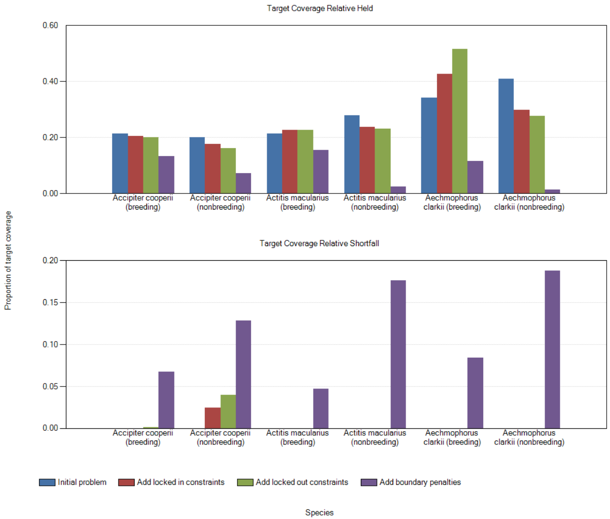
25. Lastly, double-click on the pre-configured Target coverage chart. The upper chart shows the proportion of species distributions covered by the solutions under the different scenarios. In turn, the bottom chart shows the respective deviation from the target coverage of 20%. The results point to a trade-off between the least fragmented solution (purple) and meeting the target coverage.
This tutorial demonstrated how prioritizr can be used to build spatial formulations of conservation problems. Next, to create and solve a tabular conservation problem, see the next tutorial Tabular conservation prioritization with prioritizr SyncroSim.