Getting started with ecoClassify

Here we provide a guided tutorial on ecoClassify, an open-source package for developing and applying an image classifier model.

ecoClassify is a package within the SyncroSim framework. Familiarity with SyncroSim is helpful but not required to follow this tutorial. Throughout the Quickstart tutorial, terminology associated with SyncroSim is italicized, and whenever possible, links are provided to the SyncroSim online documentation. For more on SyncroSim, please refer to the SyncroSim Overview and Quickstart tutorial.

ecoClassify Quickstart Tutorial

This quickstart tutorial will introduce you to the basics of working with ecoClassify. The steps include:

1. Installing ecoClassify
2. Opening a configured ecoClassify library
3. Viewing model inputs
4. Running models
5. Viewing model outputs and results

Step 1: Installing ecoClassify

Before we begin, you must have SyncroSim Studio and the ecoClassify package installed. Download the latest stable release of SyncroSim Studio here and follow the installation prompts.

Open SyncroSim Studio and select File > Local Packages. This will open the Local Packages window in the main panel of SyncroSim Studio. In the bottom left corner, click on Install from Server…, select ecoClassify from the window that opens, and click OK.

If you do not have Miniconda installed on your computer, a dialog box will open asking if you would like to install Miniconda. Click Yes. Once Miniconda is done installing, a dialog box will open asking if you would like to create a new conda environment. Click Yes. Note that the process of installing Miniconda and the ecoClassify conda environment can take several minutes. If you choose not to install the conda environment you will need to manually install all required package dependencies.

Miniconda is an installer for conda, a package environment manager that installs any required packages and their dependencies. By default, ecoClassify runs conda to install, create, save, and load the required environment for running ecoClassify. The ecoClassify environment includes R and Python software and associated packages.

Step 2: Opening a configured ecoClassify library

Having installed the ecoClassify package, you are now ready to create your SyncroSim library. A library is a file (with extension .ssim) that contains all your model inputs and outputs. Note that the layout of each library is specific to the package for which it was initially created. You can opt to create an empty library or download the ecoClassify template library in SyncroSim Studio. In this tutorial, we will be working with the ecoClassify template library.

Start SyncroSim Studio by searching for it using the Windows toolbar and under the file menu, select Open. Once SyncroSim Studio opens, navigate to File > New and select From Online Template….

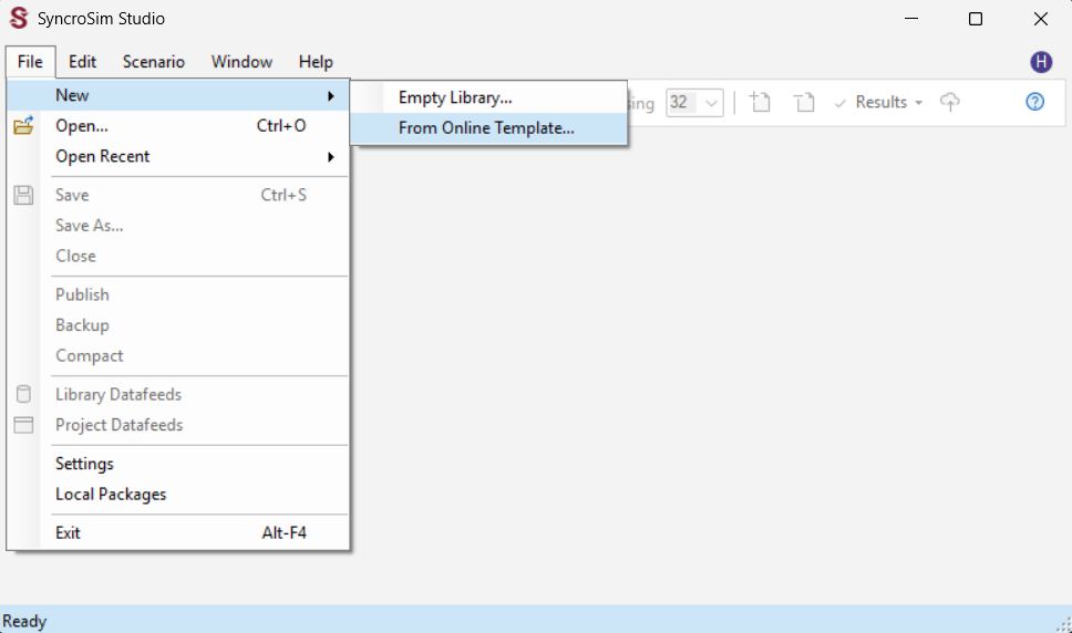
Select the ecoClassify package. Notice that the only available template is the ecoClassify Example. Select C:\Temp\ as the destination folder and click OK. The ecoClassify example will automatically open in the SyncroSim Studio explorer.

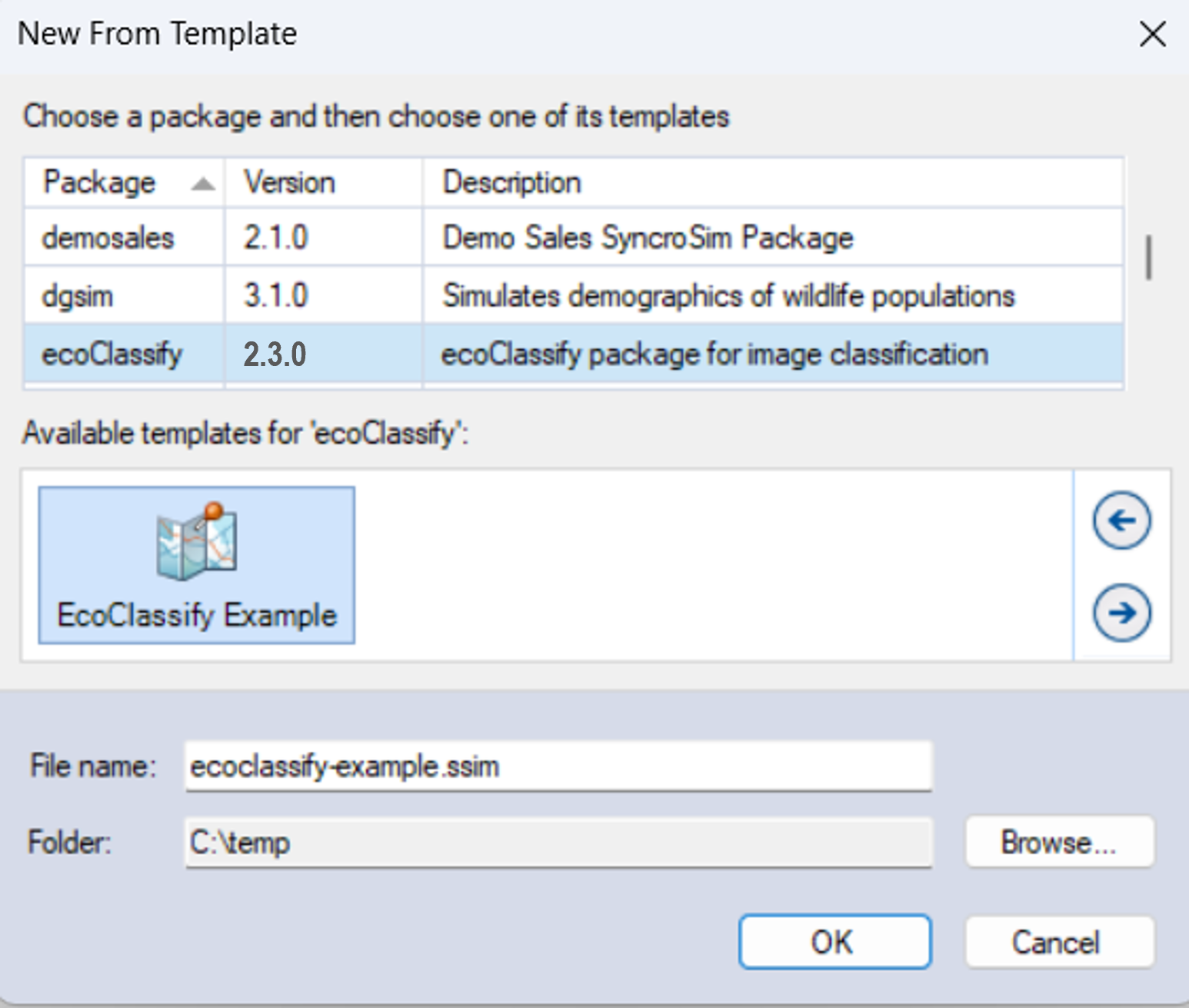
The ecoClassify example library was created with SyncroSim Studio v3.1.20. If you have a more recent release of SyncroSim Studio installed, you will automatically be prompted to update the library to configure it to your installed version of the software. Click Apply.

Step 3: Viewing model inputs

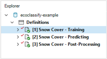
The contents of your newly opened library are now displayed in the Library Explorer. The library stores information on three levels: the library, the project, and the scenarios.

Most model inputs in SyncroSim Studio are organized into scenarios, where each scenario consists of a suite of properties, one for each of the model’s required inputs. Because you downloaded and opened a complete ecoClassify library, your library already contains three demonstration scenarios with pre-configured model inputs and outputs. In this tutorial’ we’ll work through the Snow Cover - Training, Snow Cover - Predicting, and Snow Cover - Post-Processing scenarios, demonstrating each of the three steps in the ecoClassify pipeline.

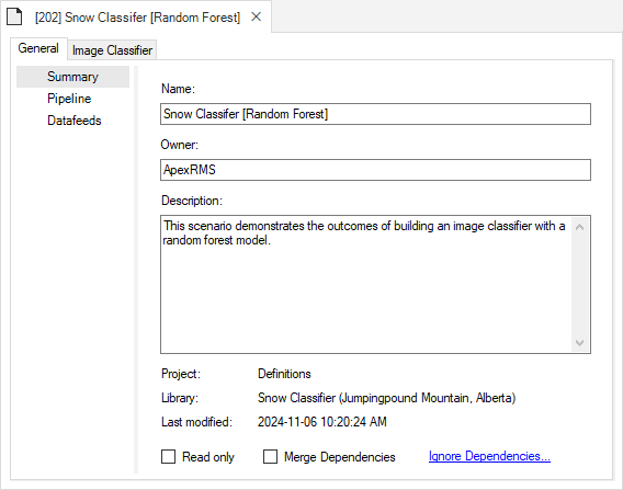
To view the details of the scenario:

• Select the scenario named Snow Cover - Training in the Library Explorer.
• Right-click and choose Open from the context menu, or double-click on the scenario.

This opens the scenario properties window.

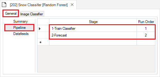
Pipeline

Located underneath the General tab, the model Pipeline allows you to select which stages of the model to include and in what order they should be run. A full run of ecoClassify consists of three stages:

• (1) Train Classifier: builds a model using training rasters and ground-truth data
• (2) Predict: applies the trained model to classify new rasters
• (3) Post-Process: filters or reclassifies the training and prediction outputs

Note that the Predict stage is dependent on the results of the previous stage, Train Classifier, and the Post-Process stage is dependent on the Train Classifier and Predict stages. You cannot run a stage without having first run the previous required stages, either within the same scenario or included as dependencies.

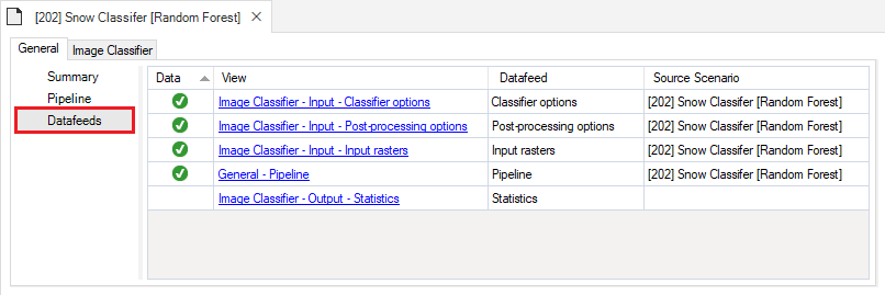
Next, click on the Datafeeds node. Here, all of the inputs to the model are listed as individual datasheets. Notice how some rows have a green checkmark in the Data column to indicate these datasheets contain data. From here, you can navigate to these individual datasheets by clicking on their name in the View column, or by navigating to the next tab called Image Classifier.

Stage 1: Training

Input

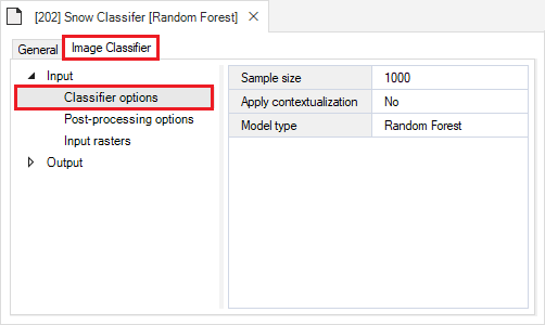
The first node under the ecoClassify tab is the Input node. Expand this node to reveal the following input datasheets:

• Classifier options
• Rasters
• Advanced

The Classifier options datasheet is where you may specify a sample size and and choose from a drop-down menu of model types. Model types currently available include Random Forest, Convolutional Neural Network (CNN), and MaxEnt. In this example training scenario we use a Random Forest model.

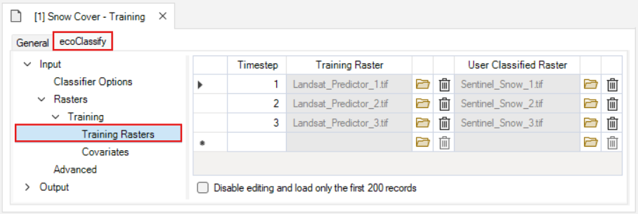
The Rasters tab contains two datasheets, Training Rasters and Covariates.

The Training Rasters datasheet is where training and user classified spatial data are loaded into the library. Note that this datasheet also contains a Timestep column. In the ecoClassify package, timesteps are used to link training rasters with their corresponding user classified rasters.

The Covariates datasheet is where additional spatial data are loaded into the library. Note that there is no Timestep column; these data are applied to each timestep.

The Advanced datasheet contains several sections that control how the model is trained and tuned.

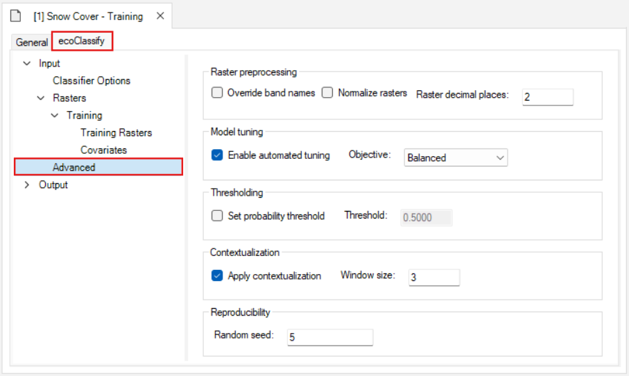
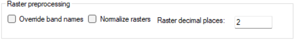
Raster preprocessing:

• Selecting Normalize Rasters applies min-max normalization to each training raster in the Training Rasters datasheet to have values ranging between 0 and 1.
• Adjusting the Raster decimal places value specifies the number of decimal places assigned to the values in each pixel. Reducing the number of decimal places can reduce the memory disk space required to process large rasters.

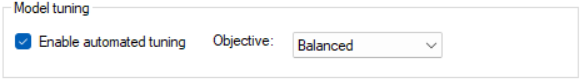
Model tuning:

• Selecting Enable automated tuning tunes the model to optimize for the Objective that is specified.
  • For Random Forest models, multiple combinations of hyperparameters (mtry, maxDepth, and nTrees) are evaluated in parallel, and the best model is selected based on the lowest OOB error. If not enabled, default hyperparameters are used.
  • Maxent Models are also evaluated with hyperparameter tuning, and the best model is selected based on Continuous Boyce Index (CBI).
  • For CNN models, a greater number of epochs and a larger batch size are used to evaluate the model when automated tuning is enabled.
• Selecting a model tuning Objective maximizes the specified objective (choose between Youden, Accuracy, Specificity, Sensitivity, Precision, and Balanced) within minimum metric constraints.

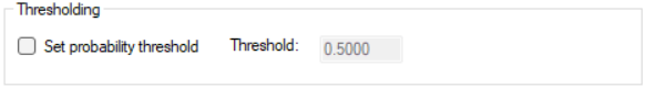
Thresholding:

• Selecting Set probability threshold switches to manually setting a probability threshold for classifying a pixel as present or absent rather than the default of automated probability threshold selection.
• Adjusting the Threshold value defines the manual probability threshold.

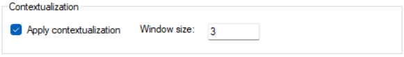
Contextualization:

• Selecting Apply contextualization applies spatial contextualization to the list of training rasters by computing local statistics and principal components over a square moving window.
• Adjusting the Window size defines the contextualization window size. This value must be an odd number.

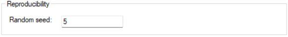
Reproducibility:

• Adjusting the Random seed value fixes the starting point of the random number sequence used for sampling the training rasters.

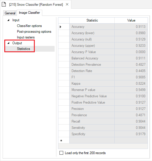
Output

Finally, the Output node contains the Statistics datasheet. This datasheet is filled with key statistics for the image classifier model that is generated during the Training step. To view an example, click on the drop-down arrow to the left of the Snow Cover - Training scenario and double click on the Snow Cover - Training result scenario and navigate to the Statistics datasheet.

Stage 2: Predicting

Next, right click on the scenario named Snow Cover - Predicting in the Library Explorer and choose Open from the context menu, or double-click on the scenario.

Navigating to the Pipeline datasheet under the General tab shows that the 2-Predict stage is used in this scenario.

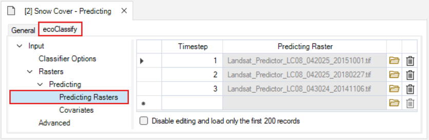
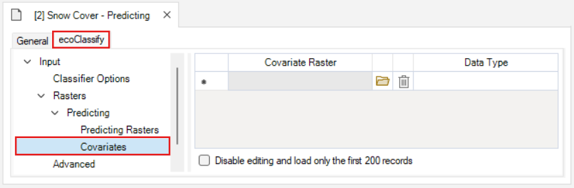
Input

In the 2-Predict stage, there is a new Predicting tab under Input > Rasters. This tab contains two new datasheets: Predicting Rasters and Covariates.

The Predicting Rasters datasheet is where rasters to be classified are loaded into the library. As with the Training rasters datasheet, this datasheet also contains a Timestep column to provide a unique identifier for each predicting raster. These rasters must have layer names that match the names used to train the image classifer.

The Covariates datasheet is where additional spatial data are loaded into the library. Note that these data are applied to each timestep, and their layer names must match the names used to train the image classifer.

Stage 3: Post-Processing

Right click on the scenario named Snow Cover - Post-Processing in the Library Explorer and choose Open from the context menu, or double-click on the scenario.

The Pipeline datasheet under the General tab shows that the 3-Post-Process stage is used in this scenario.

Post-Processing Options

The Post-Process stage has a new Post-Processing Options tab with two datasheets: Filtering and Rule-Based Restrictions.

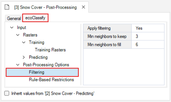
The Filtering datasheet contains options for filtering and filling in the classified rasters.

• Selecting Apply filtering enables the filtering feature for all classified rasters generated from Stage 1 and 2.
• The Min neighbours to keep value specifies the threshold for the number adjacent present pixels required in order to not filter out the central pixel. A higher value results in more filtering.
• the Min neighbours to fill value specifies the threshold for the number adjacent present pixels required in order for the pixels surrounding the central pixel to be reclassified as present. A higher value results in less filling.

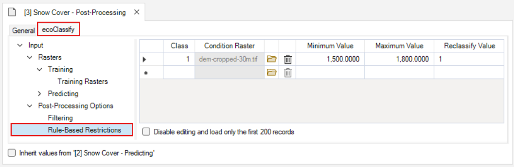
The Rule-Based Restrictions datasheet is where you can apply rules for reclassifying the rasters based on the pixel values in supplied rasters with the same resolution and spatial extent.

• The Class value specifies the class that the reclassification rules should be applied to (0 or 1).
• The Condition Raster is where you can load the raster containing values that the rules are based on.
• The Minimum Value is the lowest value in the range of rules.
• The Maximum Value is the highest value in the range of rules.
• The Reclassify Value is the value that should be assigned to pixels that fall within the specified range.

In this example, the pixels are assigned a value of 1 (present) in the classified raster where values in the dem-cropped-30m.tif raster have a value between 1500-1800:

Dependencies

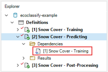
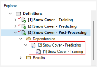
Dependencies can be used to break each stage up into a separate scenario, as is done in this example library. Click on the drop-down icon on the left side of the Snow Cover - Predicting scenario to show the two nested folders: Dependencies and Results. Click on the Dependencies folder. The first scenario, Snow Cover - Training, is present as a dependency. The most recent results from this scenario will be used as the inputs to the Predicting scenario each time it is run.

Click on the Dependencies folder in the Snow Cover - Post-Processing scenario; the Snow Cover - Predicting scenario is present as a dependency, and the Snow Cover - Training dependency for the predicting scenario is included as well.

Step 4: Running models

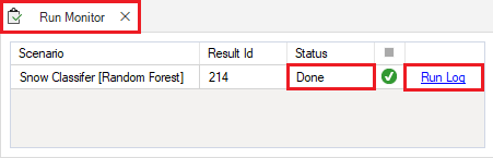
Right-click on the Snow Cover - Training scenario in the Library Explorer window and select Run from the context menu. If prompted to save your project, click Yes. The example model run should complete within a couple of minutes. If the run is successful, you will see a Status of Done in the Run Monitor window. If the run fails, you can click on the Run Log link to see a report of any problems that occurred. A blue information symbol indicates that there is additional information in the run log, which will occur in all scenarios using the Training stage.

Repeat for each of the two remaining scenarios, Snow Cover - Predicting and Snow Cover - Post-Processing.

Step 5: Viewing model outputs and results

Once the run is complete, you can view the details of the result scenario:

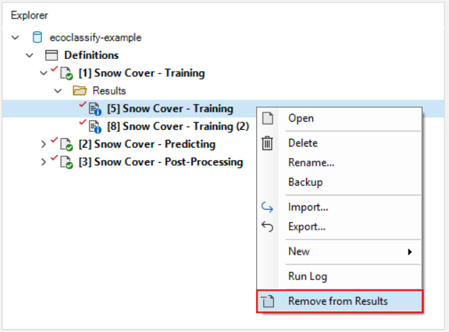
• In the Library Explorer, expand the drop-down arrow next to the Snow Cover - Training scenario to reveal the Results folder. Nested under this folder are the result scenarios. Note that this template ecoClassify library already contains results, which is why there are two result scenarios associated with this parent scenario.

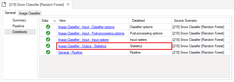
• Right-click and choose Open from the context menu to view the details of the result scenario you just produced. This opens the result scenario properties window. The format of the result scenario properties is similar to the scenario properties but contains read-only datasheets with updated information produced during the model run. Notice how the output Statistics datasheet now appears in the results scenario’s Datafeeds.

You can look through the result scenario to see the updated or newly populated datasheets. You should find that the Output datasheet, Statistics, has been populated with model run outputs.

Charts

To view tabular outputs, move to the results panel at the bottom left of the Library Explorer window. Under the Charts tab, double-click on the Model Fit chart to view the accuracy metrics from the model training results.

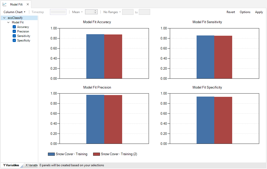
Note: results can be added or removed from the maps and charts by right clicking on the scenario and selecting “Add to/Remove from Results” in the context window.

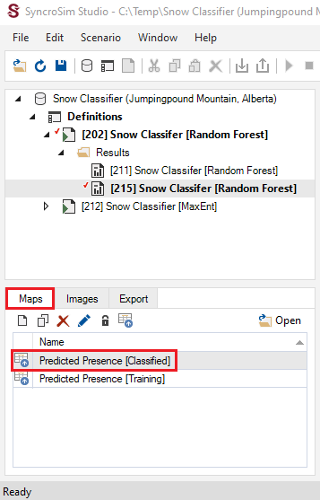
Maps

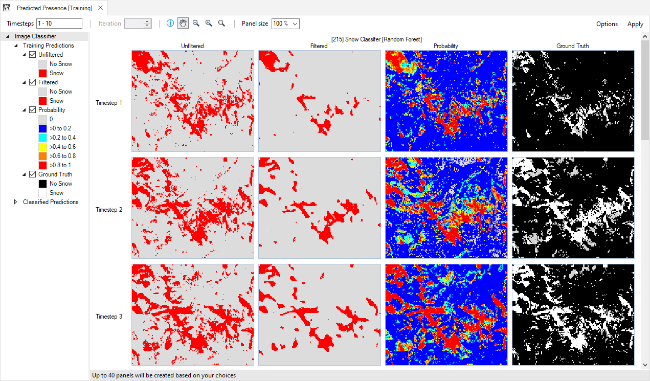
To view spatial outputs, move to the Maps tab and double-click on the Training map to visualize the classified rasters.

In order, the columns show the User Classification map (true presence), Probability map, and Binary map. The Binary (Filtered), Binary (Restricted), and Binary (Restricted and Filtered) columns will be populated with results from the Snow Cover - Post-Processing scenario. Scroll through the map page to see the Post-Processed results.

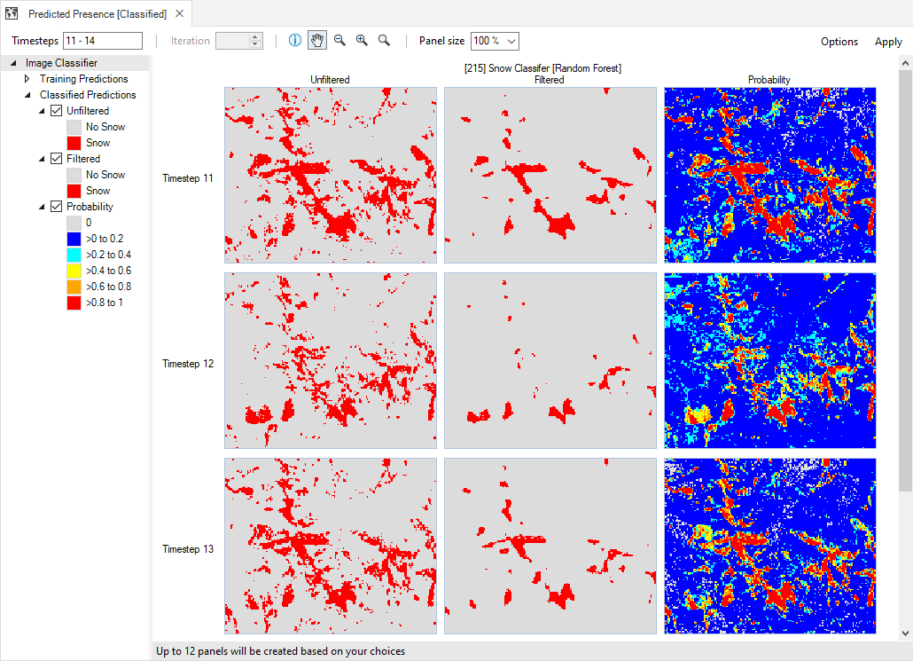
Next, double-click on the Predicting map to view the Probability and Binary panels for the Snow Cover - Predicting results scenario. Note that the Binary (Restricted), Binary (Filtered), and Binary (Restricted and Filtered) results of the training rasters will be populated with results from the Snow Cover - Post-Processing scenario. Scroll through the map page to see the Post-Processed results:

Images

ecoClassify also allows you to visualize the RGB images of your classified and training rasters under the Images tab.

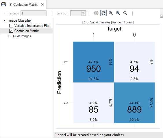
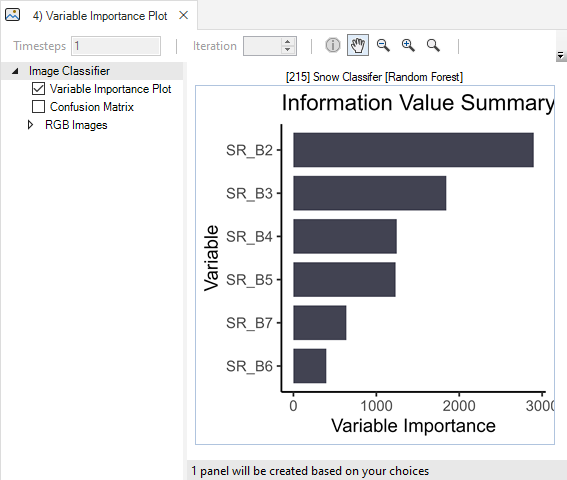
Here, you may also view a confusion matrix quantifying the classifier’s performance, a bar chart of the classifier’s variable importance, and a Histogram for each training variable overlaid with the model response.

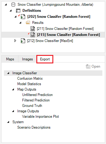
Export Data

To export model outputs, add the result scenario with the desired outputs to the results and open the Export tab at the bottom of the screen. All available files for export will be listed. To export, simply double-click on the desired output and choose the directory in which to save the file in the pop-up window. Note that if multiple result scenarios are included in the active result scenarios, files for each of the selected scenarios will be exported.