Getting started with LUCAS Builder
Quickstart Tutorial
This quickstart tutorial will introduce you to the basics of working with LUCAS Builder. The steps include:
- Installing LUCAS Builder
- Creating a LUCAS Builder Library from a template
- Viewing model inputs and outputs
- Running the model
Step 1: Install LUCAS Builder
LUCAS Builder is a package within the Syncrosim simulation modeling framework, and requires SyncroSim Studio to be installed on your computer. Download and install SyncroSim 3.1.9 or later.
To install the LUCAS Builder package, open SyncroSim and select File > Local Packages > Install from Server…, select the lucasbuilder package and click OK. Repeat the process to install the stsim package. Visit the ST-Sim documentation page for additional information on ST-Sim.
If you do not have Miniforge installed on your computer, a dialog box will open asking if you would like to install Miniforge. Click Yes. Once Miniforge is installed, a dialog box will open asking if you would like to create a new conda environment. Click Yes. Note that the process of installing Miniforge and the lucasbuilder conda environment can take several minutes. If you choose not to install the conda environment, you will need to install R version 4.1.3 or later.
Miniforge is an installer for conda, a package environment manager that installs any required packages and their dependencies. By default, lucasbuilder runs conda to install, create, save, and load the required environment for running LUCAS Builder, including the R software and necessary packages.
Note: The LUCAS Builder package includes a template library, LUCAS Builder - CONUS, that contains example inputs and outputs. Installation of conda or R is not required to view the Template Library inputs and outputs.
Step 2: Create a new LUCAS Builder Library
Having installed the LUCAS Builder package, you are now ready to create your first SyncroSim Library. A Library is a file (with extension .ssim) that contains all of your model inputs and outputs. The format of each library is specific to the Package for which it was initially created. You can opt to create an empty library or download the lucasbuilder template library. In this tutorial, we will be using the the LUCAS Builder - CONUS template library.
- Go to File > New > From Online Template…
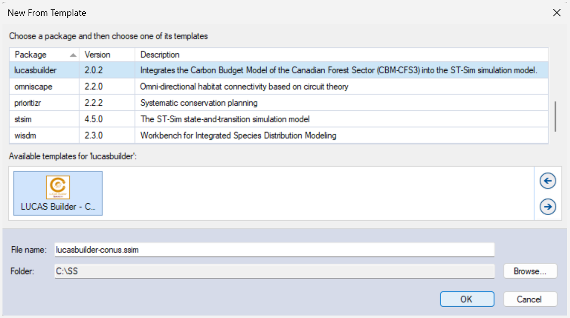
In this window: - Select the row for lucasbuilder. Note that as you select a row, the list of Templates available and suggested File name for that base package are updated.
- Select the LUCAS Builder - CONUS template as shown above.
- Optionally, type in a new File name for the library (or accept the default); you can also change the target Folder using the Browse… button.
Note: If you intend on using Multiprocessing (recommended), ensure your SyncroSim library is saved to a drive that is not being synchronized to the cloud. Saving your library to OneDrive, Dropbox or some other similar location can result in an error when completing a model run.
When you are ready to create the library file, click OK. A new library will be created and loaded into the library Explorer.
Step 3: Review the model inputs and outputs
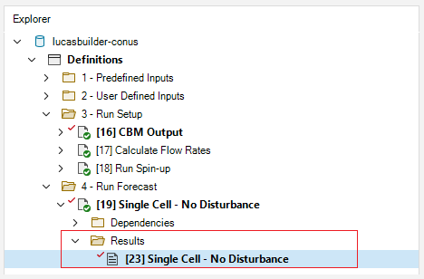
The contents of the template library are now displayed in the Explorer. Model inputs in SyncroSim are organized into Scenarios, where each scenario consists of a suite of values, one for each of the model’s required inputs.
Because you chose the LUCAS Builder - CONUS template when you created your library, it already contains four folders:
- 1 - Predefined Inputs
- 2 - User Defined Inputs
- 3 - Run Setup
- 4 - Run Forecast
The Predefined Inputs folder contains pre-configured scenarios that act as inputs for the Run Setup and Run Forecast scenarios. The User Defined Inputs folder contains two sub-folders (Run Setup Inputs and Run Forecast Inputs) that house user input scenarios that need to be populated before running the Run Setup and Run Forecast scenarios.
Note: The User Defined Inputs have been populated to provide an executable example to help you get started quickly.
In the User Defined Inputs folder, select and review the inputs for the scenarios in the Run Setup Inputs sub-folder.
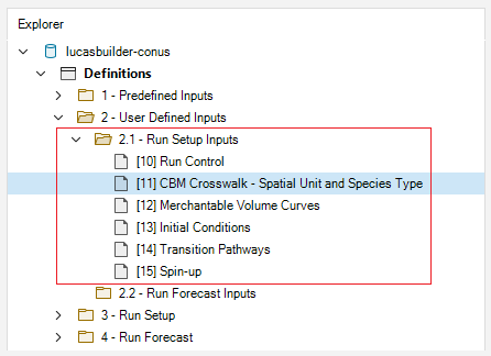
- Select the Scenario named CBM Crosswalk – Spatial Unit and Species Type in the Explorer.
- Double-click to open the scenario and view its details.
This opens the scenario Properties window. The first tab in this window, called General, contains three datasheets. The first, Summary, displays some general information for the scenario. The second, Pipeline, allows the user to select the run order of the inputs in the model. Finally, the Datafeeds datasheet (shown below) displays a list of all data sources, where each data source is a datafeed, a collection of one or more datasheets.
- Select the CBM Crosswalk to ST-Sim – Spatial Unit and Species Type datafeed to view the example inputs.
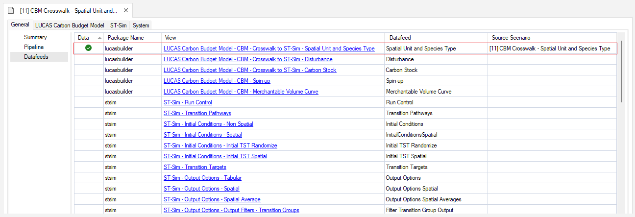
Note: Populated datasheets will appear at the top of the Datafeeds list with a green check mark in the Data field.
The crosswalk datasheet allows a user to associate each forest type to a carbon budget model (CBM) equivalent combination of Ecological Boundary, Administrative Boundary, and Species Type. Here a user can specify temperature values that should be used when modeling dead organic matter transfer and decay rates. Note that if temperature values are not specified, the default values for the selected Ecological Boundary will be used. Optionally, a user can load CBM output files, which can be compared against simulations run in ST-Sim for validation purposes (see below).
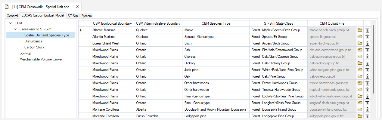
Note: In the example, the ST-Sim Stratum, ST-Sim Secondary Stratum, and Average Temperature columns have been populated and hidden for image clarity. In a custom library, users will need to manually set values for these columns.
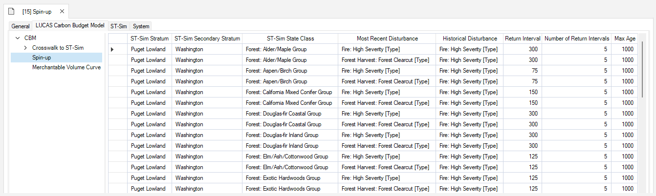
- Select the scenario named Spin-up in the Explorer and navigate to the Spin-up datasheet.
We see that each ST-Sim State Class defined in the species crosswalk has been linked with each transition (disturbance) type.
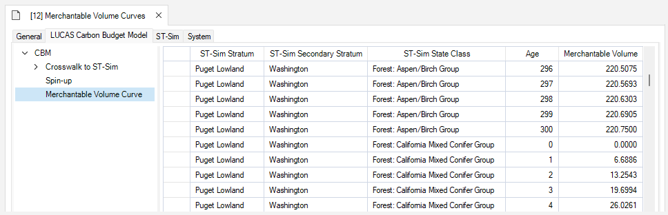
- Select the Merchantable Volume Curve scenario and navigate to the Merchantable Volume Curve datasheet.
Merchantable volume curves need to be added to the Merchantable Volume Curve scenario for each ST-Sim State Class defined in the species crosswalk. Note that editing is disabled for this datasheet in the template library, but this can be enabled again.
When all scenarios in the User Defined Inputs folder are populated, the Run Setup scenarios can be run.
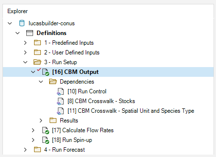
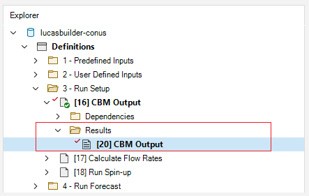
Click on the scenarios in the Run Setup and Run Forecast folders to view the scenario dependencies and familiarize yourself with each scenario’s inputs. The CBM Output scenario has already been run, so you will also see a Results folder within this scenario.
- Open the CBM Output scenario and select Pipeline from the General tab.
Notice that only the first stage, 1 - Load CBM Output, has been selected for this scenario. This stage serves to build results based on the standard CBM-CFS approach, and is optional in your analysis.
- Select Datafeeds from the General tab to see the scenario’s active datasheets.
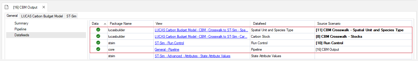
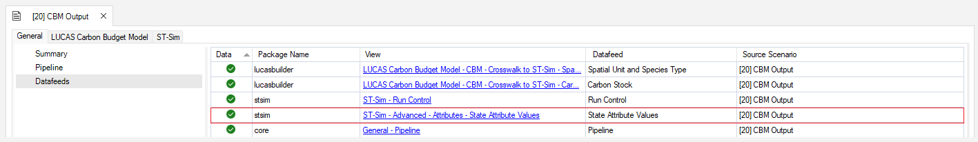
- Open the Result Scenario for CBM Output.
Looking at Datafeeds, notice that the State Attribute Values datasheet was populated as a result of running the CBM Output scenario.
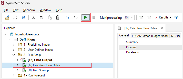
Following the steps above, view the Pipeline and input and output Datafeeds for the Calculate Flow Rates and Run Spin-up scenarios.
Step 4: Run the model
If not using conda, SyncroSim needs the location of your R executable, which will be found automatically if it is installed in the default location. To check, double-click on the lucasbuilder-conus library and navigate to the System tab. In the Tools > R datasheet, you should see the file path to your R executable. If not, click Browse… and navigate to the correct file location.
- Select the Calculate Flow Rates scenario and press Run on the top toolbar. If prompted to save your library, click Yes.
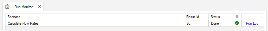
If the run is successful, you will see a Status of Done in the Run Monitor window, at which point you can close the Run Monitor window; otherwise, click on the Run Log link to see a report of any problems. Make any necessary changes to your scenario, then re-run the scenario.
- Repeat the process with the Run Spin-up scenario.
Notice that the outputs from the Calculate Flow Rates scenario serve as inputs for the spin-up runs. In turn, the results from the Run Spin-up scenario are used as inputs for the Single Cell – No Disturbance scenario. Looking at the Pipeline of each scenario, you can notice the sequence of modeling stages.
Warning Note: Running these scenarios will take approximately 3.5 GB of disk space.
Once the Run Setup scenarios have completed successfully, the Run Forecast scenario can be run.
- Repeat the steps above to run the Single Cell – No Disturbance scenario.
When a scenario is run, a new Result Scenario will appear in the Results folder, and its results are automatically loaded after a successful scenario run. Scenarios which contain results added to the results viewer appear in bold in the Explorer.
You can add and remove Result Scenarios from the list of scenarios being analyzed by selecting a scenario in the Explorer and then choosing Add to Results or Remove from Results from either the Scenario menu tab, or by right-clicking over the scenario. To simplify the outputs, right-click over the Calculate Flow Rates and Run Spin-up scenarios and select Remove from Results at the bottom of the menu.
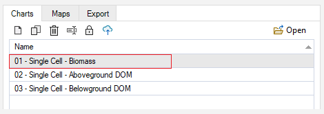
Scenario results can be viewed and compared through Charts and Maps. You can compare the results of your Single Cell – No Disturbance run with validation outputs generated by the CBM Output scenario by adding both scenarios to the Results Viewer.
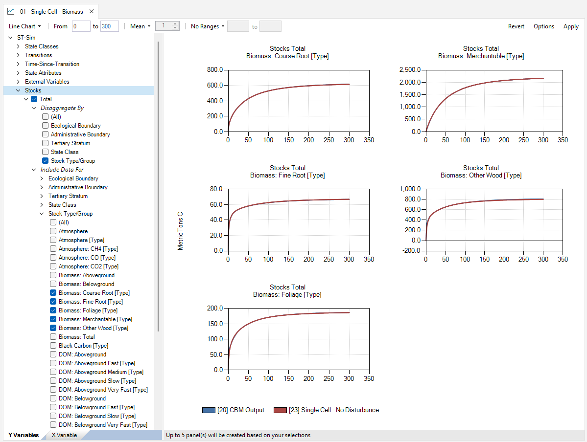
- Move to the Charts tab at the bottom left of the Scenario Manager screen and double-click on the Single Cell – Biomass chart to open it.
The following charts will be plotted. The two colours correspond to the two scenarios that were added to the Results Viewer.
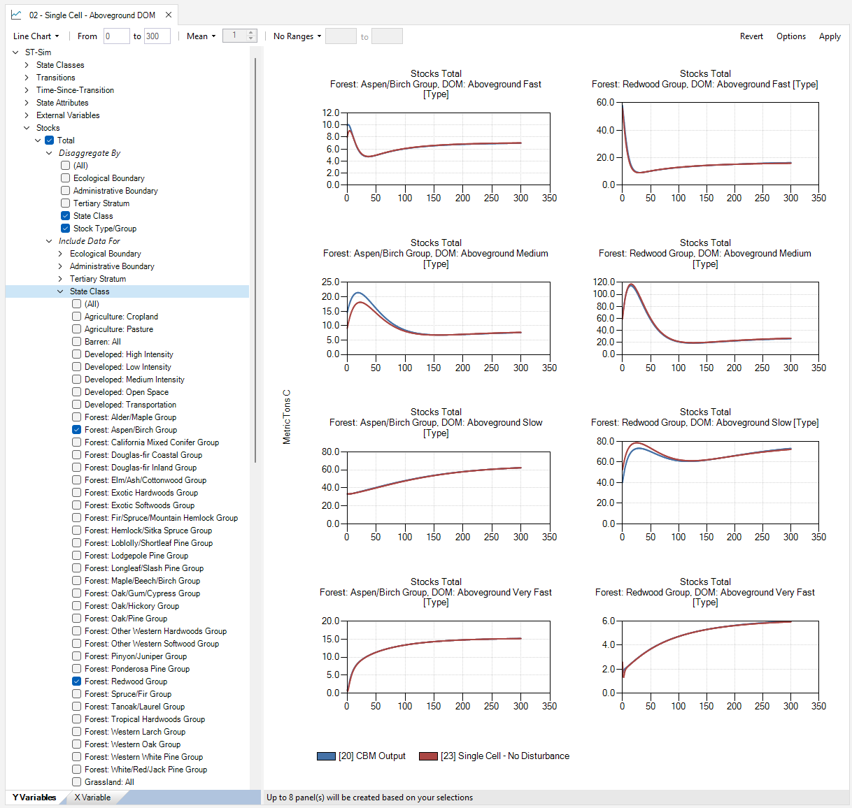
- Double-click on the Single Cell – Aboveground DOM and Single Cell – Belowground DOM charts to view the results.
You can view results for the different forest types by changing the State Class selection and then clicking Apply.
Note: This example is non-spatial. Therefore, there are no map outputs to display.
The Single Cell – No Disturbance scenario differs slightly from the CBM Output for some forest types. These discrepancies are due to different default input parameter values in the CBM output. For example, in this LUCAS Builder – CONUS template library, we used a fire return interval of 1000 years for the Redwoods Forest Type Group, whereas the CBM output used a default fire return interval of 300 years. Also, LUCAS Builder uses a different smoothing algorithm for nonmerchantable biomass pools at young stand ages; therefore, results from the LUCAS Builder package will differ slightly from the CBM output at young stand ages.