Climate refugia prioritization with prioritizr SyncroSim
This tutorial provides an overview of working with prioritizr in SyncroSim Studio to create a simplified version of a climate-refugia prioritization approach that explores the effects of different criteria and feature weighing schemes on the results. It covers the following steps:
Step 1. Creating a prioritizr SyncroSim library
In SyncroSim, a library is a file with extension .ssim that stores all the model’s inputs and outputs in a format specific to a given package. To load the pre-configured library:
1. Open SyncroSim Studio.
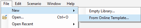
2. Select File > New > From Online Template….
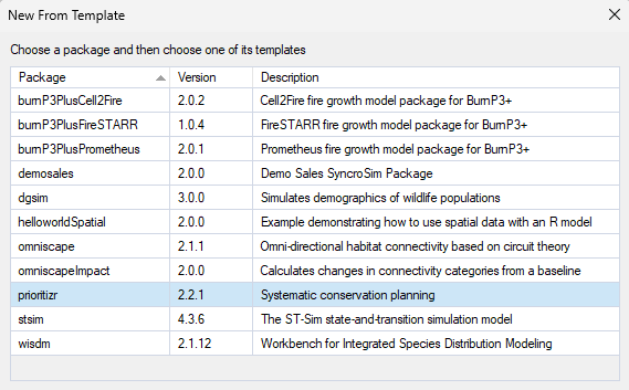
b. From the list of template libraries, select Climate Refugia Prioritization (Muskoka, Ontario).
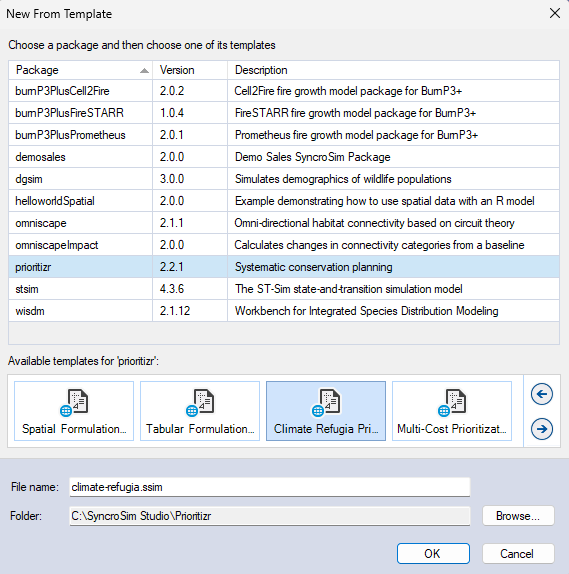
c. If desired, you may edit the File name, and change the Folder by clicking on the Browse button.
d. When done, click OK.
A new library has been created based on the selected template, and SyncroSim will have automatically opened and displayed it in the Explorer window.
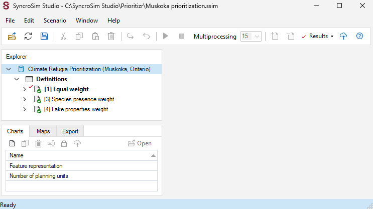
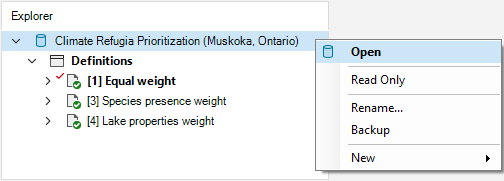
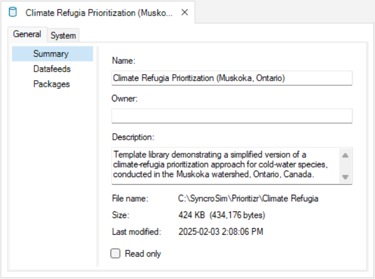
3. Double-click on the library name, Climate Refugia Prioritization (Muskoka, Ontario), to open the library properties window. You may also right-click on the library name and select Open from the context menu.
4. The Summary datasheet contains the metadata for the library.
5. Next, navigate to the Systems tab, Options node, General datasheet, and make sure Use conda is disabled.
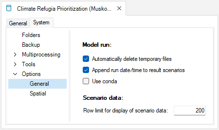
6. Close the library properties window.
Next, you will review the target feature data for the conservation prioritization problem.
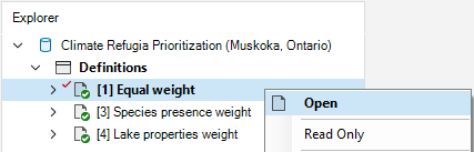
7. From the Explorer window, right-click on Definitions and select Open from the context menu.
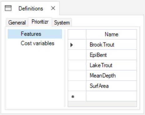
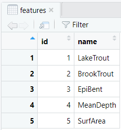
8. Under the Prioritizr tab, select the Features datasheet, which lists the variables that will be taken into account in the prioritization process. Here, the feature data corresponds to three lake property variables (i.e., Epi-benthic Habitat, Mean Depth, and Surface Area) and two species occurence records (i.e., for Brook Trout and Lake Trout). This datasheet was automatically populated once the first scenario was run.
Now you will review the inputs for the Equal weight scenario, which provides a baseline where all features have the same weight. In SyncroSim, each scenario contains the model inputs associated with a model run.
9. In the Explorer window, select the pre-configured scenario Equal weight and double-click it to open its properties. You may also right-click on the scenario name and select Open from the context menu.
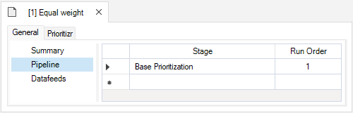
10. Navigate to the Pipeline datasheet. Pipeline stages call on a transformer (i.e., script) which takes the inputs from SyncroSim, runs a model, and returns the results to SyncroSim. Under the Stage column, note that a single pipeline stage is set called Base Prioritization.
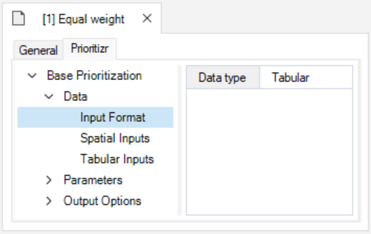
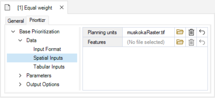
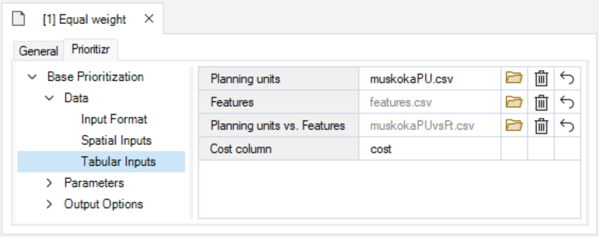
11. Navigate to the Prioritizr tab and expand the Base Prioritization > Data nodes.
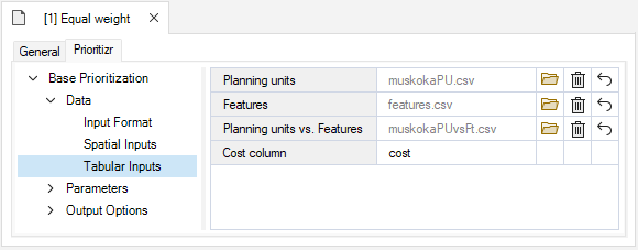
ii. Features – a data table listing the feature variables. These are listed under the column name, with an associated ID.
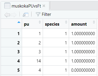
iii. Planning units vs. Features – a data table listing for each lake (under the pu column), the value (under the amount column) associated with each feature variable (under the species column).
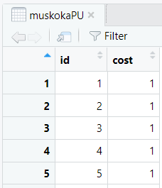
iv. Cost column – corresponds to the column in the Planning units input representing the cost variable.
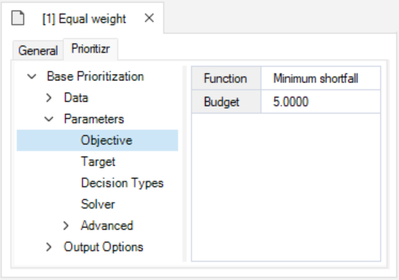
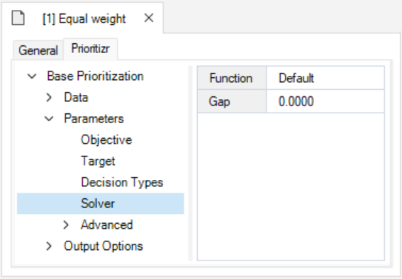
12. Expand the Parameters node.
ii. Budget – this number represents the maximum allowed cost of the prioritization. Here, the budget is used to ensure that 30% of lakes in the study area are represented in the solution, which corresponds to 5.
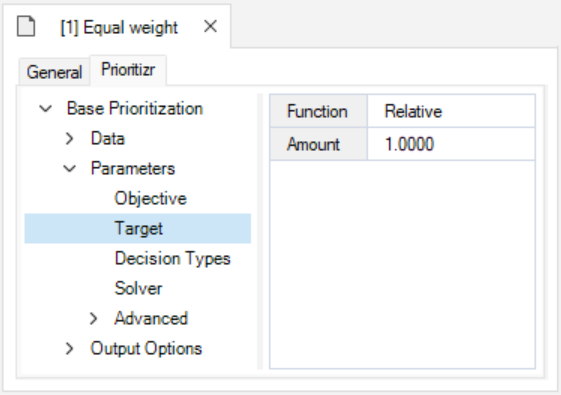
ii. Amount – specifies the desired level of feature representation in the study area. In this example, it is set to 1.0, so that each feature would ideally have 100% of its distribution covered by the prioritization.
ii. Gap – represents the gap to optimality and is set to a value of 0. This gap is relative and expresses the acceptable deviance from the optimal objective. In this example, a value of 0 will result in the solver only stopping when it has found the best possible solution.
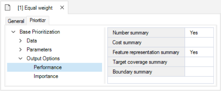
13. Expand the Output Options node and open the Performance datasheet to review the following inputs set to Yes:
ii. Feature representation summary – calculates how well features are represented by the solution to the conservation planning problem.
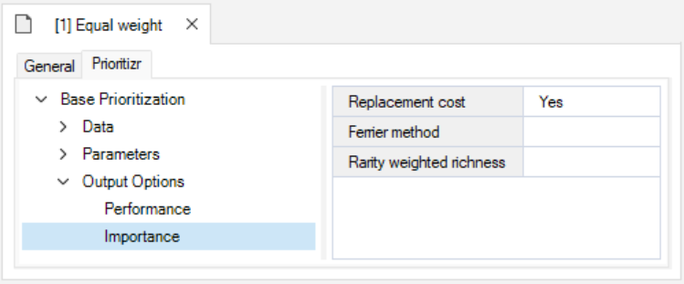
14. Open the Importance datasheet to review the following inputs set to Yes:
Step 2. Visualizing and comparing results across scenarios
The Climate Refugia Prioritization (Muskoka, Ontario) template library already contains the results for each scenario. Before exploring additional scenarios, you will view the main results for the Equal Weight scenario.
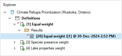
1. In the Explorer window, expand the Equal weight > Results nodes to reveal the Equal weight result scenario. This scenario contains the outputs of the model run, it is timestamped, and has a copy of all the input parameters.
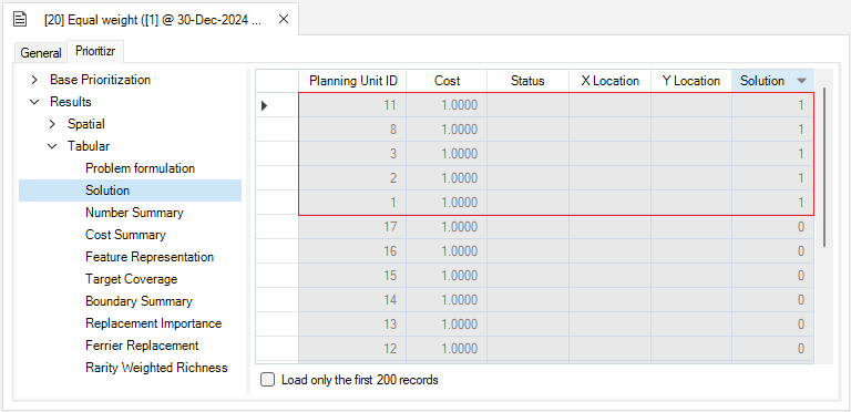
2. Double-click on the Equal weight result scenario to open its properties. You may also right-click it and select Open from the context menu.
b. Click on the Solution column to reorder the table's contents in decreasing order. Solution values equal to 1 represent the planning units that were selected by the solution.
3. Close the scenario properties tab, and from the Explorer window, collapse the scenario node by clicking on the downward facing arrow beside the Equal weight scenario.
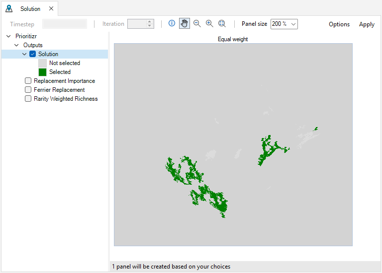
4. Navigate to the Maps tab, and double-click on the pre-configured Solution map. This map displays a visual representation of the tabular result you just inspected, showing the lakes that were selected in the solution to the conservation planning problem.
5. Close the results panels.
Now, you will review the additional scenarios, which are equal to the Equal weight scenario for all but one input: the Feature weights. Feature weights are an advanced way of controling the relative importance of different features in the prioritization process.
6. In the Explorer window, select the pre-configured scenario Species presence weight and double-click it to open its properties. You may also right-click on the scenario name and select Open from the context menu.
7. Navigate to the Prioritizr tab, expand the Advanced node, and open the Feature weights datasheet to review the following inputs:
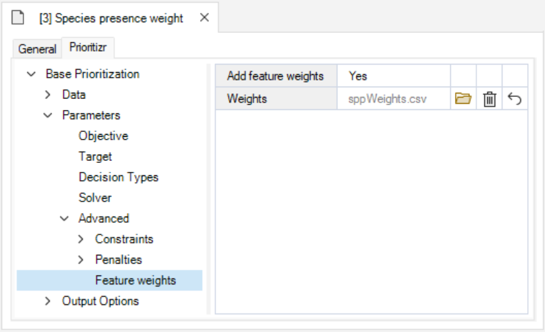
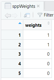
b. Weights – a data table outlining the weight of feature. From Step 1.c.ii, recall that features 1 and 2 represent the species presence features LakeTrout and BrookTrout. Here, both species presence variables have the same weight of 1, and all lake property variables have a weight of 0. In essence, this means that in this scenario, only the species presence features will be considered in the prioritization process, and will be treated with equal importance.
8. In the Explorer window, select the pre-configured scenario Lake properties weights and double-click it to open its properties.
9. Navigate to the Prioritizr tab, expand the Advanced node, and open the Feature weights datasheet to note the input Weights. Here, both species presence variables now have a weight of 0, and all lake property variables have the same weight of 1. In essence, this means that in this scenario, only the lake property features will be considered in the prioritization process.

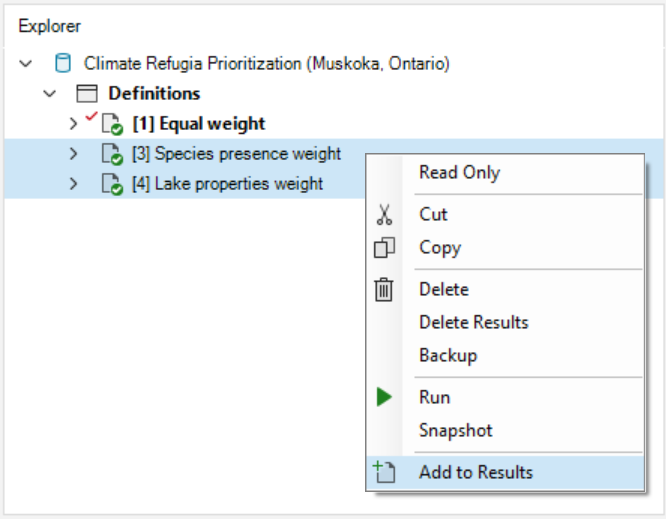
10. In the Explorer window, select scenarios Species presence weight and Lake properties weights, right-click and select Add to Results from the context menu.
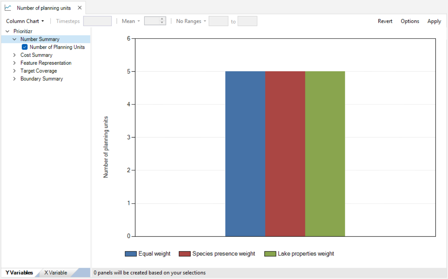
11. Navigate to the Charts tab, and double-click on the pre-configured Number of planning units chart. This chart displays the total number of planning units in the solution per scenario. In this example, 5 lakes were selected in the solution, showing the budget was met in all three scenarios.
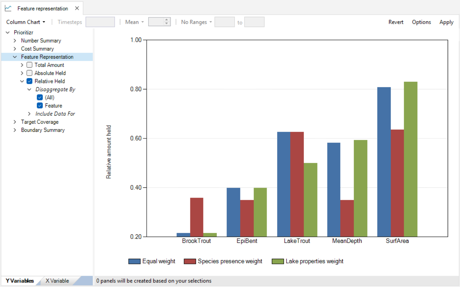
12. Next, double-click on the pre-configured Feature representation chart. This chart shows the effect of the feature weights on the proportion of each feature secured within the solution. Note that feature representation for the species presences features (i.e., BrookTrout and LakeTrout) are generally higher under the Species presence weight scenario, and the lake property features (i.e., EpiBent, MeanDepth and SurfArea) are generally higher under the Lake properties weights scenario.
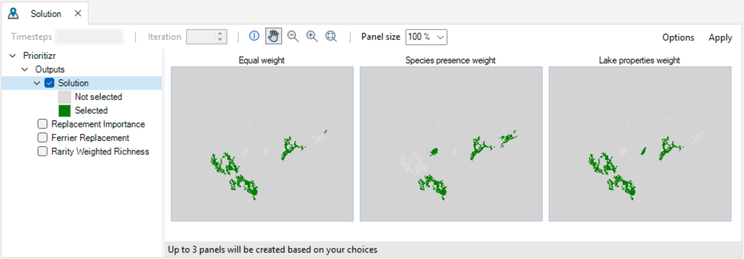
13. Next, navigate to the Maps tab, and double-click on the pre-configured Solution map. This map displays the lakes that were selected in the solution under each scenario. Note that some lakes were selected in every scenario.
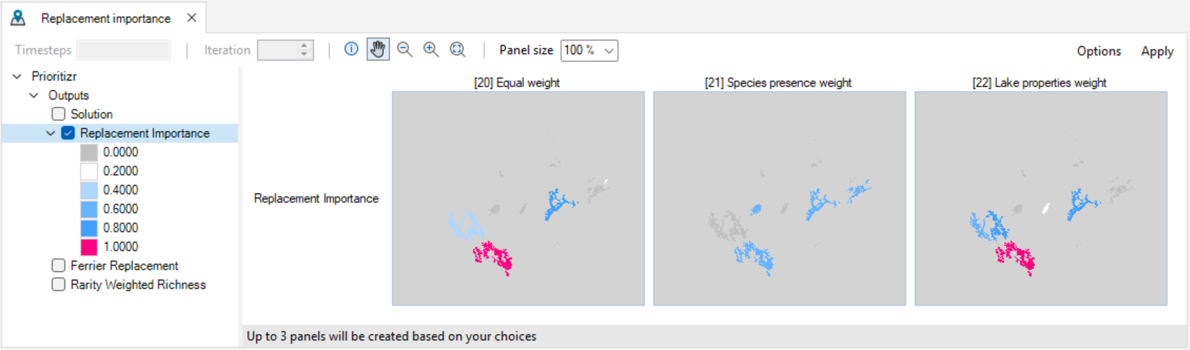
15. Finally, double-click on the pre-configured Replacement importance map. This map displays the importance scores for each lake selected in the solution based on the replacement cost method. Note that the lakes that were always selected also tended to have higher scores.
This tutorial demonstrated how prioritizr can be used to build tabular formulations of conservation problems, with a spatial visualization of the results, and covered how to add feature weights to control the relative importance of features in the prioritization. Next, to explore how to further customize a conservation problem with multiple cost layers, see the next tutorial Multi-Cost Prioritization with prioritizr SyncroSim.