Getting started with ST-Sim CBM-CFS3
Quickstart Tutorial
This quickstart tutorial will introduce you to the basics of working with ST-Sim CBM-CFS3. The steps include:
- Installing ST-Sim CBM-CFS3
- Creating a new ST-Sim CBM-CFS3 Library
- Viewing model inputs and outputs
- Running the model
Step 1: Install ST-Sim CBM-CFS3
ST-Sim CBM-CFS3 is a Package within the Syncrosim simulation modeling framework; as such, ST-Sim CBM-CFS3 requires that the SyncroSim software be installed on your computer. Download and install SyncroSim 2.3.11 or later here.
If you choose to run ST-Sim CBM-CFS3, you will also need to install the CBM-CFS3 and R version 4.0.2 or later.
Note: The ST-Sim CBM-CFS3 package includes two template Libraries, CBM-CFS3 Example and CBM-CFS3 CONUS, that contain example inputs and outputs. Installation of R and the CBM-CFS3 are not required to view the template Libraries.
Once all required programs are installed, open SyncroSim and select File -> Packages… -> Install… and select the stsim, stsimsf, and stsimcbmcfs3 packages and click OK.
Please refer to the documentation for additional information on ST-Sim and the Stock-Flow add-on packages (stsim and stsimsf).
Step 2: Create a new ST-Sim CBM-CFS3 Library
Having installed the ST-Sim CBM-CFS3 Package, you are now ready to create your first SyncroSim Library. A Library is a file (with extension .ssim) that contains all of your model inputs and outputs. The format of each Library is specific to the Package for which it was initially created. To create a new Library, choose New Library… from the File menu.
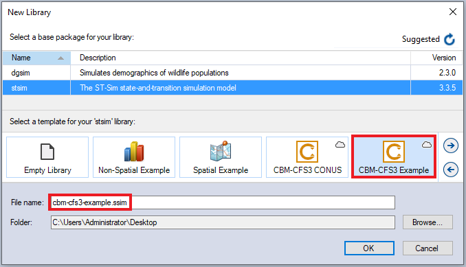
In this window:
- Select the row for stsim. Note that as you select a row, the list of Templates available and suggested File name for that base package are updated.
- Select the CBM-CFS3 Example Template as shown above.
- Optionally type in a new File name for the Library (or accept the default); you can also change the target Folder using the Browse… button.
Note: If you intend on using Multiprocessing (recommended), ensure your SyncroSim Library is saved to a drive that is not being syncronized to the cloud. Saving your library to OneDrive, Dropbox or some other similar location can result in an error when completing a model run.
When you are ready to create the Library file, click OK. A new Library will be created and loaded into the Library Explorer.
Step 3: Review the model inputs and outputs
The contents of your newly created Library are now displayed in the Library Explorer. Model inputs in SyncroSim are organized into Scenarios, where each Scenario consists of a suite of values, one for each of the Model’s required inputs.
Because you chose the CBM-CFS3 Example template when you created your Library, your Library already contains four folders:
- 1 - Predefined Inputs
- 2 - User Defined Inputs
- 3 - Run Setup
- 4 - Run Forecast
The Predefined Inputs folder contains pre-configured Scenarios that act as inputs for the Run Setup and Run Forecast Scenarios. The User Defined Inputs folder contains two sub-folders (Run Setup Inputs and Run Forecast Inputs) that house user input Scenarios that need to be populated before running the Run Setup and Run Forecast Scenarios.
Note: The User Defined Inputs have been populated to provide an executable example to help you get started quickly.
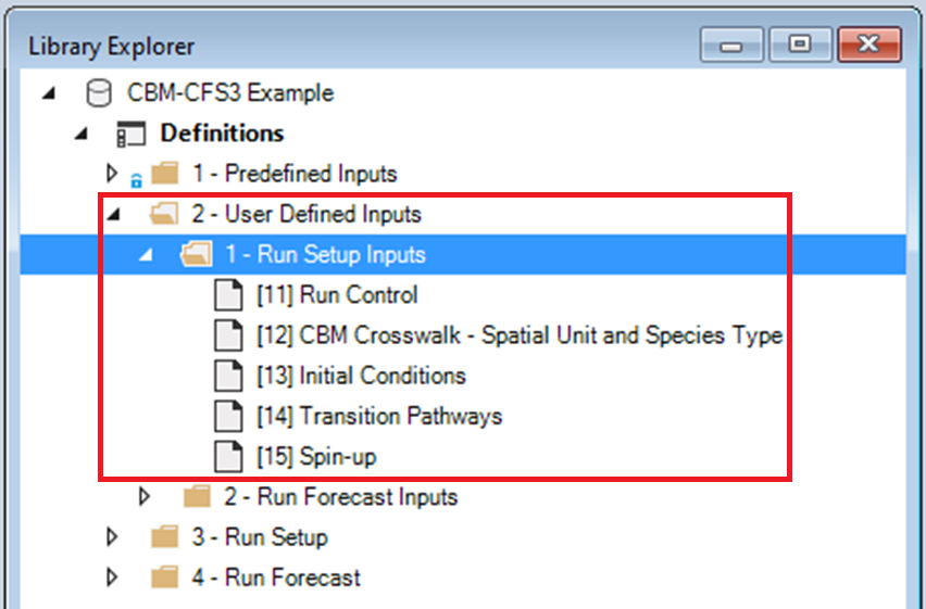
In the User Defined Inputs folder, select and review the inputs for the Scenarios in the Run Setup Inputs sub-folder.
- Select the Scenario named CBM Crosswalk – Spatial Unit and Species Type in the Library Explorer.
- Right-click and choose Properties from the context menu to view the details of the Scenario.
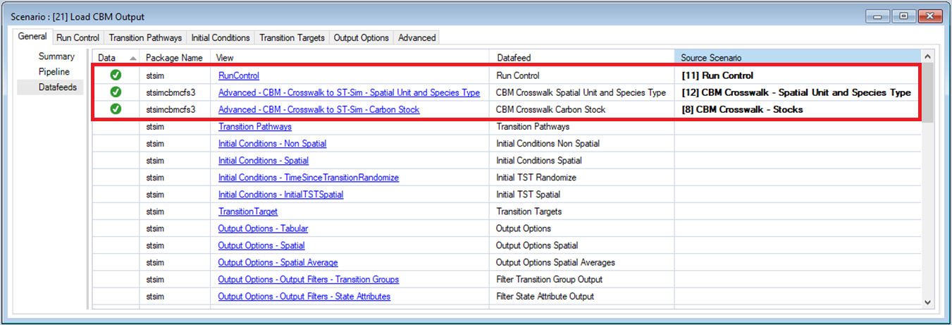
This opens the Scenario Properties window. The first tab in this window, called General, contains three datasheets. The first, Summary, displays some general information for the Scenario. The second, Pipeline, allows the user to select the run order of the inputs in the model. Finally, the Datafeeds datasheet (shown below) displays a list of all data sources.
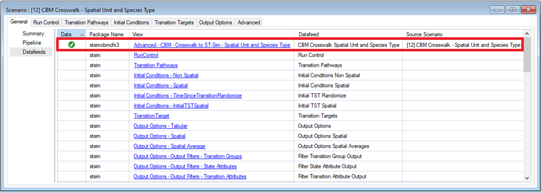
Select the CBM Crosswalk – Spatial Unit and Species Type datafeed to view the example inputs.
Note: Populated datasheets will appear at the top of the Datafeeds list with a green check mark in the Data field. This example is setup to simulate four different forest types in the Sierra Nevada Ecoregion of California:
- Western Oak,
- California Mixed Conifer,
- Ponderosa Pine, and
- Alder/Maple
The crosswalk datasheet allows a user to associate each forest type to a CBM equivalent combination of Ecological Boundary, Admin Boundary, and Species Type. Here a user can specify temperature values that should be used when modeling dead organic matter transfer and decay rates. Note that if temperature values are not specified, the default values for the selected Ecological Boundary will be used. Here a user must also load CBM output files that are used to calculate growth rates by biomass pool. Outputs loaded from the CBM can be compared against simulations run in ST-Sim for validation purposes (see below).
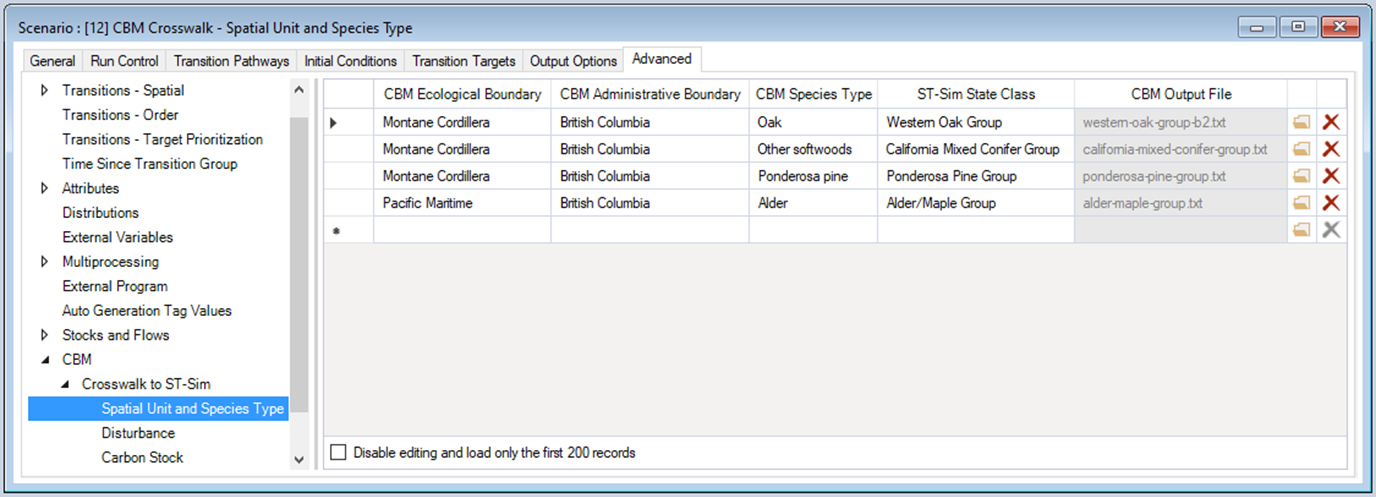
Note: In the example, the ST-Sim Stratum, ST-Sim Secondary Stratum, and Average Temperature columns have been populated and hidden for image clarity. In a custom Library, users will need to manually set values for these columns.
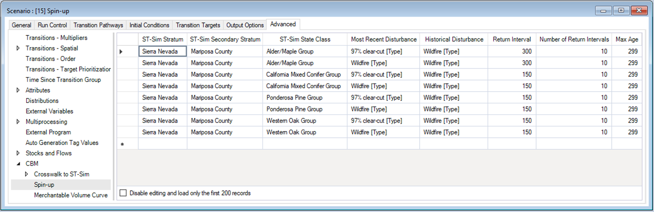
Looking at the Spin-up Scenario, we see that each ST-Sim State Class defined in the species crosswalk has been linked with each transition (disturbance) type.
When all Scenarios in the User Defined Inputs folder are populated, the Run Setup Scenarios can be run.
Click on the Scenarios in the Run Setup and Run Forecast folders to view the Scenario dependencies and familiarize yourself with each Scenario’s inputs. The Scenarios in Run Setup and Run Forecast have already been run so you will also see a Results folder when you click on each Scenario.
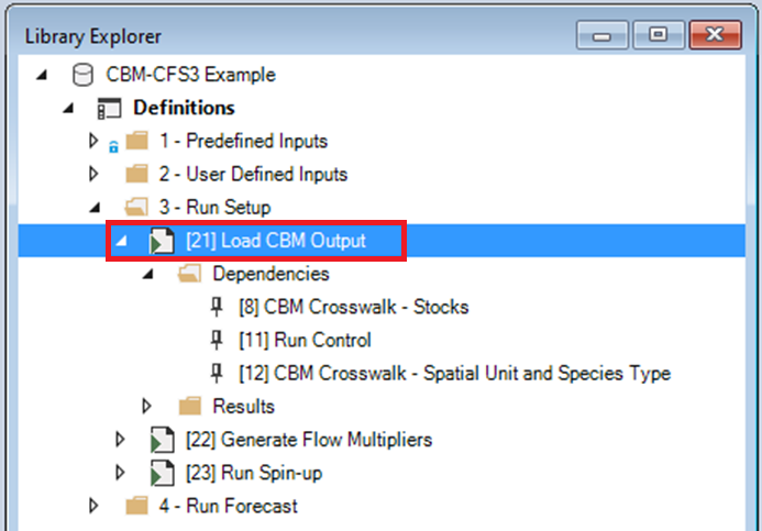
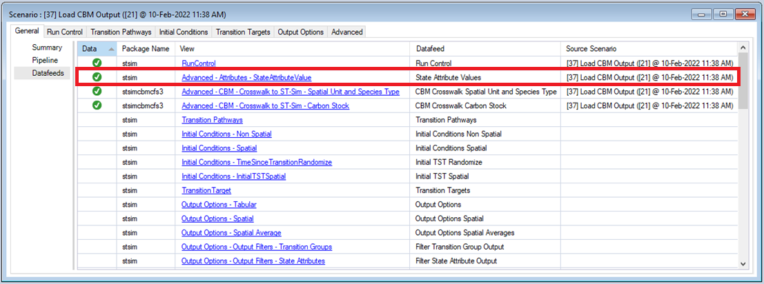
Open the Load CBM Output Scenario and select Pipeline from the General tab. Notice that, only the Load CBM Output Run Stage has been selected for this scenario. Now select Datafeeds from the General tab to see the Scenarios active datasheets.
Open the Result Scenario for Load CBM Output.
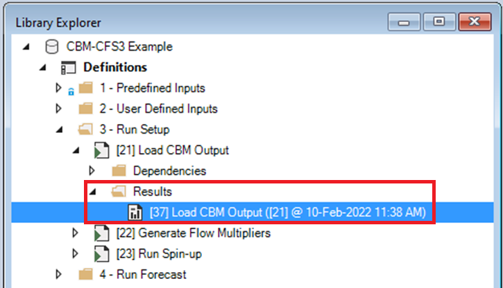
Looking at Datafeeds, notice that the State Attribute Values datasheet was populated as a result of running the Load CBM Output Scenario.
Following the steps above, view the Run Stage and input and output Datafeeds for the Generate Flow Multipliers and Run Spin-up Scenarios.
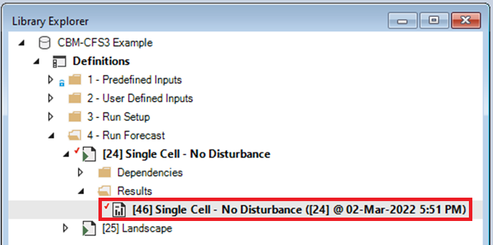
Scenario Results can also be viewed through Charts and Maps. To view results for the Single Cell – No Disturbance Scenario, select the Results Scenario in the Library Explorer and then choose Add to Results.
Note: You can add and remove Results Scenarios from the list of Scenarios being analyzed by selecting a Scenario in the Library Explorer and then choosing either Add to Results or Remove from Results from the Scenario menu. Scenarios currently selected for analysis are highlighted in bold in the Library explorer.
Next, move to the Charts tab at the bottom left of the Scenario Manager screen and double-click on the Single Cell – Biomass chart to open it.
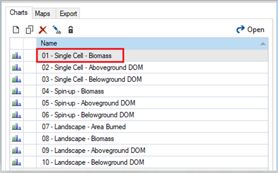
The following window should open.
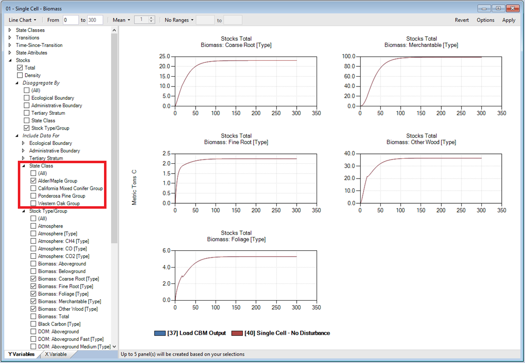
You can compare the results of your Single Cell – No Disturbance run with validation outputs generated by the Load CBM Output Scenario by adding both Scenarios to the Results Viewer.
Double-click on the Single Cell – Aboveground DOM and Single Cell – Belowground DOM charts to view the results. You can view results for the different forest types by changing the State Class selection and then clicking Apply. When done viewing the Single Cell Results, remove the Load CBM Output and Single Cell – No Disturbance Scenarios from the Results Viewer.
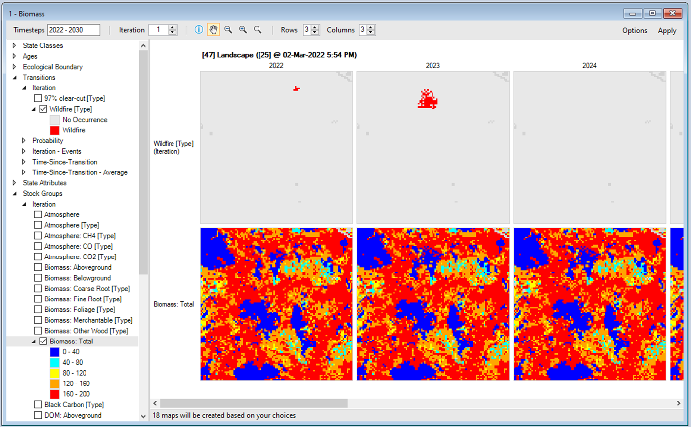
To view spatial results, add the Landscape Scenario to the Results and then select the Maps tab from the bottom of the Scenario Manager window (i.e. beside the Charts tab). Double click on the Biomass Map. By default, the mapping window should display Wildfire events and changes in Total Biomass over time.
Double click on Flows and Age Maps to view changes in carbon flows and forest age for the Landscape Scenario.
Step 5: Run the model
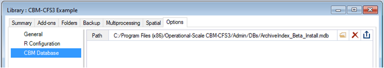
In order to run the model, SyncroSim needs the locations of your R executable and the CBM-CFS3 Database. The R executable will be found automatically. To check, double-click on CBM-CFS3 Example and navigate to the Options tab. In the R Configuration datasheet, you should see the file path to your R executable. If not, click Browse… and navigate to the correct file location. The CBM file path is set to the default location that was recommended during the installation of the database. If the CBM-CFS3 Database was not installed to the default location, select the Folder icon, and navigate to the proper location on your local computer, then click Open.
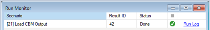
Once your CBM-CFS3 Example Library is configured, you can run the model by right-clicking on the Load CBM Output Scenario in the Scenario Manager window and selecting Run from the context menu. If prompted to save your project, click Yes. If the run is successful, you will see a Status of Done in the Run Monitor window, at which point you can close the Run Monitor window; otherwise, click on the Run Log link to see a report of any problems. Make any necessary changes to your Scenario, then re-run the Scenario.
Note: If you encounter an error in your model run, you may need to install Microsoft Access Database Engine 2016 Redistributable.
Next, repeat the steps above to run the Generate Flow Multiplier and Run Spin-up Scenarios.
Note: The Run Setup and Run Forecast Scenarios rely on dependencies that are defined in Predefined Inputs and User Defined Inputs, as well as results from previous Run Setup Scenarios. For this reason, it is important the Scenarios are run in sequence.
Once the Run Setup Scenarios have completed successfully, the Run Forecast Scenarios can be run.
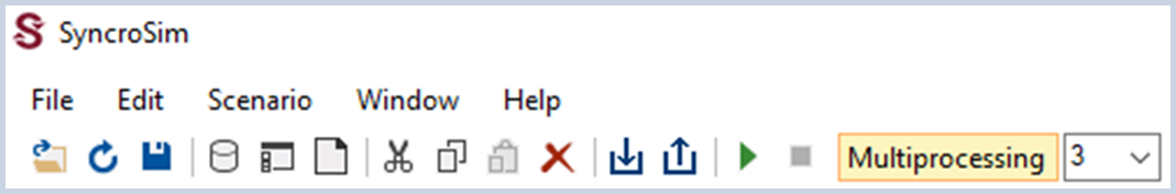
Repeat the steps above to run the Single Cell – No Disturbance and Landscape Scenarios. When running the Landscape Scenario, Multiprocessing should be enabled with 3 jobs.
When a Scenario is run, a new Results Scenario will appear in the Results folder. To view the results, select the Results Scenario in the Library Explorer and then choose Add to Results from the Scenario menu. The selected Scenario will appear in bold in the Library Explorer and the Scenario results will display in Charts and Maps.