Getting started with WISDM
Here we provide a guided tutorial on WISDM, an open-source package for developing and applying species distribution models (SDMs) and visualizing their outputs.
WISDM is a base package for SyncroSim, yet familiarity with SyncroSim is not required to get started with WISDM. Throughout the Quickstart tutorial, terminology associated with SyncroSim is italicized, and whenever possible, links are provided to the SyncroSim online documentation. For more on SyncroSim, please refer to the SyncroSim Overview and Quickstart tutorial.
WISDM Quickstart tutorial
This quickstart tutorial will introduce you to the basics of working with WISDM. The steps include:
- Installing WISDM
- Creating a new WISDM library
- Viewing model inputs
- Running models
- Viewing model outputs and results
Step 1: Installing WISDM
Running WISDM requires that the SyncroSim software be installed on your computer. Download the latest version of SyncroSim here and follow the installation prompts.
WISDM is a package within the SyncroSim simulation modeling framework. To install the WISDM package, open SyncroSim Studio and select File > Local Packages > Install from Server, then select the WISDM package and click OK.
If you do not have Miniconda installed on your computer, a dialog box will open asking if you would like to install Miniconda. Click Yes. Once Miniconda is done installing, a dialog box will open asking if you would like to create a new conda environment. Click Yes. Note that the process of installing Miniconda and the WISDM conda environment can take several minutes. If you choose not to install the conda environment you will need to manually install all required package dependencies.
Miniconda is an installer for conda, a package environment manager that installs any required packages and their dependencies. By default, WISDM runs conda to install, create, save, and load the required environment for running WISDM. The WISDM environment includes R and Python software and associated packages.
Step 2: Creating a new WISDM Library
Having installed the WISDM package, you are now ready to create your SyncroSim library. A library is a file (with extension .ssim) that contains all your model inputs and outputs. Note that the format of each library is specific to the package for which it was initially created. You can opt to create an empty library or use a template library called WISDM Example. In this tutorial, we will be working with the WISDM Example template library. To create a new library from this template, choose New… > From Online Template… > from the File menu, and selecting WISDM.
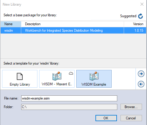
In this window:
- Select the row for wisdm - Workbench for Integrated Species Distribution Modeling. Note that as you select a row, the list of templates available and suggested File name for that package are updated.
- Select the WISDM Example template as shown above.
- Optionally type in a new File name for the library (or accept the default); you can also change the Folder containing the file using the Browse… button.
- When you are ready to create the library file, click OK. A new library will be created and loaded into the SyncroSim Studio Explorer.
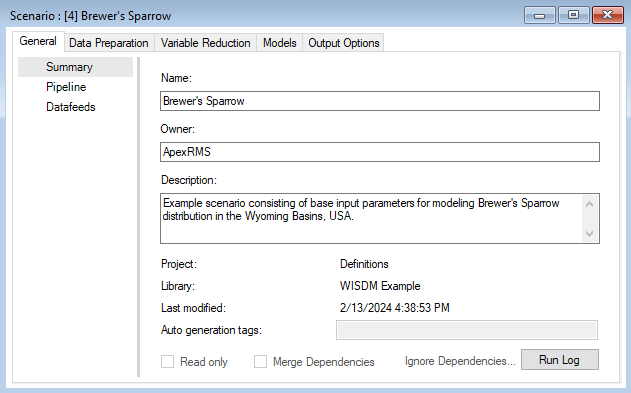
Step 3: Viewing model inputs
The contents of your newly created library are now displayed in the Explorer. The library stores information on three levels: 1.) the library, 2.) the project, and 3.) the scenario(s).
Most model inputs in SyncroSim are organized into scenarios, where each scenario consists of a suite of properties, one for each of the model’s required inputs. Because you chose the WISDM Example when you created your library, your library already contains a demonstration scenario with pre-configured model inputs and outputs.
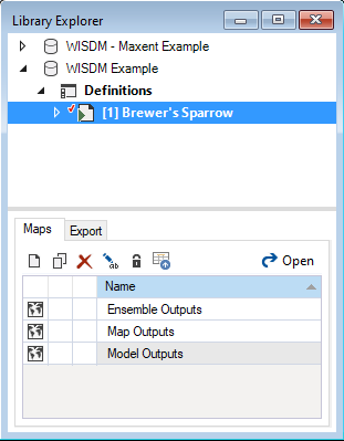
To view the details of the scenario:
- Select the scenario named Brewer’s Sparrow in the Explorer.
- Right-click and choose Open from the context menu to view the details of the scenario.
This opens the scenario properties window.
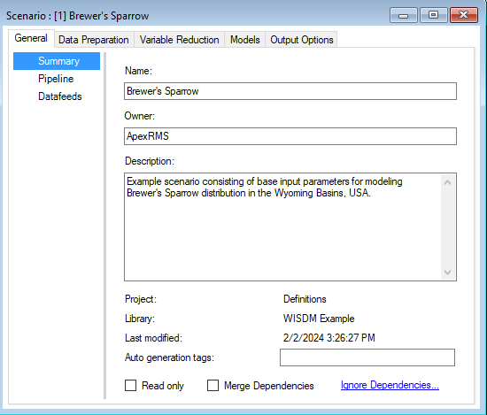
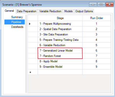
Pipeline
Located under the General tab, the model Pipeline allows you to select which stages of the model to include in the model run and their run order. A full run of WISDM consists of six to nine stages: (1) Create multiprocessing tiles (optional); (2) Prepare spatial data; (3) Prepare site data; (4) Generate background sites (optional); (5) Prepare training and testing data; (6) Variable reduction; (7) Fit statistical model(s); (8) Apply the model(s); (9) Ensemble the models (optional). The following list represents all possible Pipeline elements. In this example, however, we will only run two statistical models in Stage 7:
- Stage 1: Prepare Multiprocessing (optional)
- Stage 2: Spatial Data Preparation
- Stage 3: Site Data Preparation
- Stage 4: Background Data Generation (optional)
- Stage 5: Prepare Training/Testing data
- Stage 6: Variable Reduction
- Stage 7: Generalized Linear Model
- Stage 7: Boosted Regression Tree
- Stage 7: Random Forest
- Stage 7: Maxent
- Stage 8: Apply Model
- Stage 9: Ensemble Model (optional)
Note that all stages in this pipeline are dependent on the results of the previous stage. You cannot run a stage without having first run the previous required stages (optional stages can be skipped). However, you can choose to fit your data to any number of the statistical models available for Stage 7 (i.e., GLM, Random Forest, or Maxent). In this example, GLM and Random Forest have been selected and added to the pipeline.
Spatial multiprocessing inputs
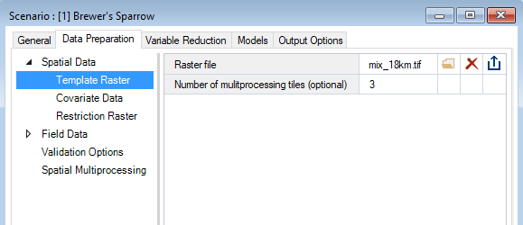
Under the WISDM > Data Preparation node, you’ll find the Template Raster datasheet. Here, you’ll provide the system path to a Raster file with the desired extent, resolution, and coordinate reference system (CRS) for the analysis and outputs. This Template Raster is required for multiple stages in the pipeline, including the optional Prepare Multiprocessing stage.
If you are choosing to run with Spatial Multiprocessing, you can also specify the Number of multiprocessing tiles that you would like to use. If you don’t specify a value, the package will select an appropriate value for you.
If spatial multiprocessing is used, a tiling raster will be created and will appear in the System > Spatial Multiprocessing datasheet when the scenario has finished running. This tiling raster is used to clip other spatial layers into smaller rectangular blocks, effectively creating more manageable processing sizes.
Note that Stage 1 (Prepare Multiprocessing) only needs to be added to the pipeline and run if spatial multiprocessing is required (i.e., for large landscapes and/or high resolution data). In this example, we will use spatial multiprocessing for demonstration purposes.
Spatial data inputs
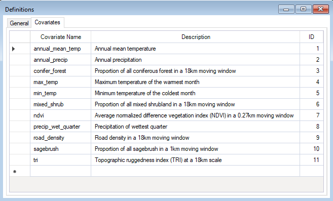
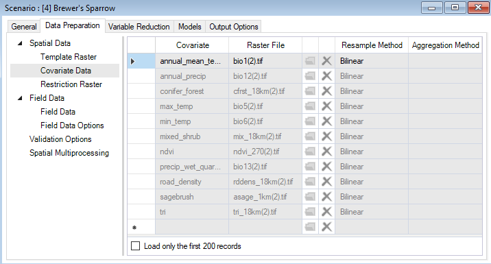
Under the Project Properties, which you can view by double-clicking in the Explorer window, in the project called Definitions, you’ll find the WISDM > Covariates datasheet. Here, you must list the names of all covariates you want to consider for model development.
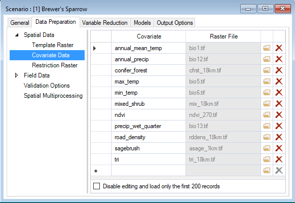
If you return to the scenario properties, under the WISDM > Data Preparation > Spatial Data node, you’ll also find a datasheet called Covariate Data. Here, you will identify system paths to the raster files (e.g., GEOTiffs) for each covariate listed in the aforementioned Covariates datasheet. The extent of each raster must be greater than or equal to the template raster extent.
Below the Covariate Data datasheet, you will see a Restriction Raster datasheet. This is an optional input, where you can specify a file path to a raster that will be used to multiply the probability raster during the apply model stage. The Restriction Raster is often binary, with the value of 0 indicating areas where occurrence probability will be reduced to zero. In addition to providing a file, you can provide a brief description of the Restriction Raster used.
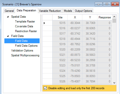
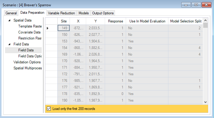
In the same Data Preparation tab, you’ll also find a Field Data datasheet. Here, you will identify site locations by their X and Y coordinates and include response values for the target species. Response values can be provided as presence-only (1), presence/absence (1 or 0), or counts (integers >= 0).
By default, WISDM assumes that the field data coordinates are provided in the template raster’s reference system. If the coordinates are provided in an alternate coordinate reference system, the corresponding authority code should be entered under the field data Field Data Options datasheet.
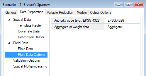
The Aggregate or weight data input gives you the option to handle redundancy and avoid pseudo-replication by either aggregating field data locations so only one field data observation is represented per pixel or proportionately down-weighting pixels with multiple points. If the input is left blank, all field data points will be retained without aggregation or weighting.
If the Background Data Generation stage is included in the scenario pipeline, the Background Data Options datasheet will be visible below the Field Data Options datasheet. Here, you can identify preferences for background site or pseudo-absence generation, such as whether background sites should be generated, the number of sites that should be generated, the method used for generation, KDE (kernel density estimation) background surface method, and the isopleth threshold used for binary mask creation. This datasheet is optional and is left blank for the purposes of this tutorial.
Field data inputs
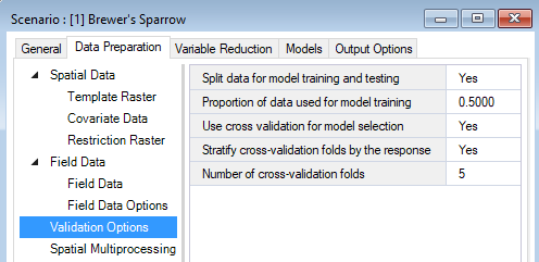
Still under the WISDM > Data Preparation tab, you’ll find the Validation Options datasheet. Here, you’ll indicate if data should be split into training and testing datasets and the proportion of data that should be used for training. If left blank all data is used for training and no data is reserved for testing. In this datasheet, you can also indicate if cross validation (CV) should be used, the number of CV folds the data should be split into (the default is 10), and if the data in the folds should be stratified by the response (i.e., relatively equal representation of the response variables in each fold). If Use cross validation for model selection is left blank, cross validation will not run.
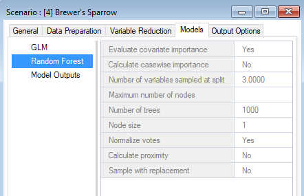
Statistical models
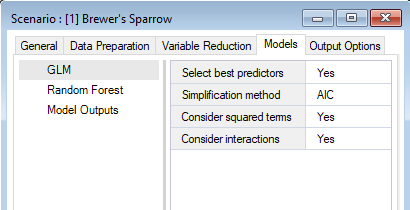
Under the WISDM > Models node, you’ll find the Generalized Linear Model, Random Forest, and Model Outputs datasheets. Depending on which statistical models you included in your pipeline, you can access the corresponding model configuration datasheet here and customize your desired statistical analysis. If fields are left blank, default values will be used.
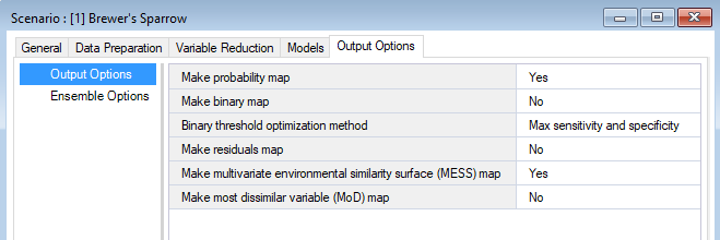
Output options
In the WISDM > Output Options datasheet, you can choose which output maps to generate. Five output options are available for selection: (1) Probability Map, (2) Binary Map, (3) Residuals Map, (4) Multivariate Environmental Similarity Surface (MESS) Map, and (5) Most Dissimilar Variable (MoD) Map. Choosing at least one option is required to produce output maps. If this datasheet is left blank, the probability map will be generated by default and all other maps will not be generated.
Step 4: Running models
Right-click on the Brewer’s Sparrow Scenario and select Run from the context menu. If prompted to save your library, click Yes.
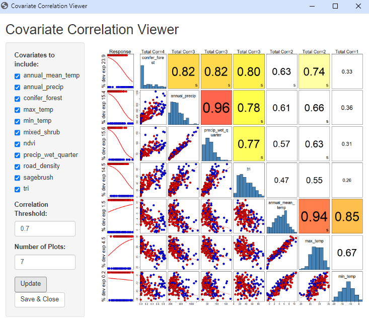
During the model run, the Covariate Correlation Viewer window will open in your default browser, showing correlations between Covariates. Here, you can manually remove covariates from consideration based on user interpretation (e.g., if the correlation values are deemed unacceptable). To remove a Covariate, uncheck the box next to the variable name in the Covariates to include list. A default threshold correlation absolute value of 0.7 (highest of Spearman, Pearson, Kendall) is used to color code the correlation values. This value, and the number of plots shown, can be changed. To view changes, simply select the Update button. Once you are satisfied with your list of covariates, select the Save & Close button. The window will close and the analysis will continue in Syncrosim.
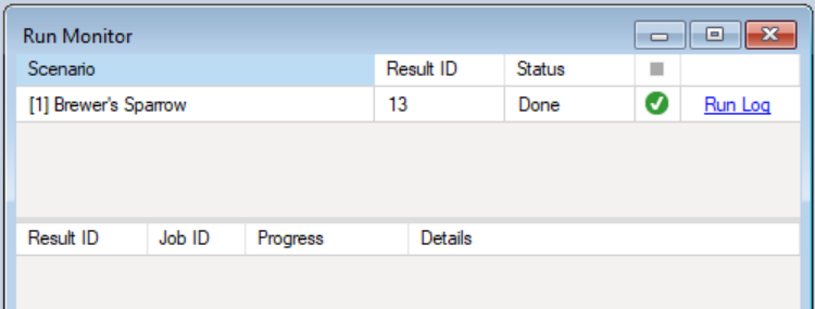
The example model run should complete within a couple of minutes. If the run is successful, you will see a Status of Done in the Run Monitor window. If the run fails, you can click on the Run Log link to see a report of any problems that occurred.
Step 5: Viewing model outputs and results
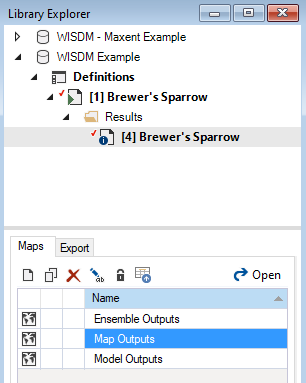
Once the run is complete, you can view the details of the Results Scenario:
- Select Brewer’s Sparrow Results Scenario from the Results folder nested under the Brewer’s Sparrow Scenario in the Library Explorer.
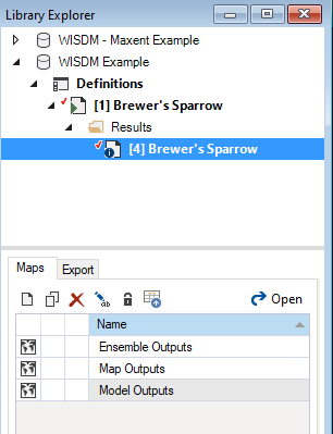
- Right-click and choose Open from the context menu to view the details of the results scenario.
This opens the Results Scenario Properties window. The format of the Results Scenario Properties is similar to the Scenario Properties but contains read-only datasheets with updated information produced during the model run.
You can look through the results scenario to see the updated or newly populated datasheets. You should find that the Field Data, Covariate Data, GLM, and Random Forest datasheets have updated entries. Note that the model configuration options for Random Forest were left empty in the Parent Scenario. In this case, WISDM uses default settings during model fitting and reports the selections in the results scenario.
Data preparation outputs
The Field Data datasheet has also been updated to only include training data and background (pseudo-absence) sites inside the extent of the template raster. In the Options datasheet, if weight was selected, the Weights column will also be populated. If aggregate was selected, records with -9999 may occur in the Response column, this indicates redundancy, and these records will be removed from model fitting. The Use In Model Evaluation and Model Selection Split columns will also be populated based on selections defined in the Validation Options datasheet. The Use in Model Evaluation column indicates which sites were used for model training and testing. A Yes in this column means that the site was reserved for model evaluation (i.e., testing) and was not used during model fitting (i.e., training). The Model Selection Split column indicates how the training data has been spilt for cross validation. This column is only populated if Use cross validation for model selection was chosen under Validation Options, and will display the cross-validation fold assigned to each site.
Back in the Covariate Data datasheet, you’ll find that all your input rasters have been replaced by clipped, reprojected, and resampled rasters that match the properties of your Template Raster (extent, CRS, spatial resolution). The Resample Method and Aggregation Method columns have been populated with default values to indicate which approach was used to prepare the data.
In the results scenario you should also find that the Spatial Multiprocessing datasheet under the Data Preparation tab has been populated, along with the Site Data and Retained Covariate List datasheets under the Variable Reduction tab.
Since we opted for multiprocessing, we can see that a tiling raster has been created and added to the Spatial Multiprocessing datasheet. This tiling raster is used to clip other spatial layers into smaller rectangular blocks, effectively creating more manageable processing sizes.
Site Data is an output of the Site Data Preparation stage of the Pipeline and provides site specific values for each covariate. The Retained Covariate List is an output of the Variable Reduction stage of the Pipeline and lists the candidate variables that were considered during model fitting.
Model outputs
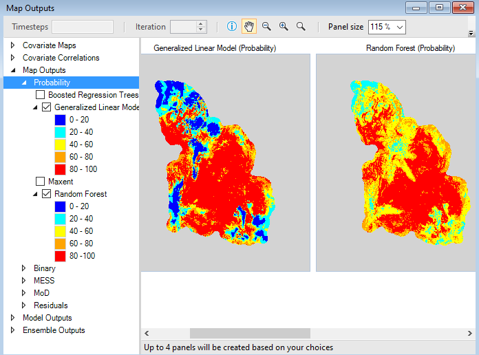
To view spatial outputs, move to the results panel at the bottom left of the Explorer window. Under the Maps tab, double-click on Map Outputs to visualize the map.
The first two maps are Probability maps showing model-predicted habitat suitability values in geographic space. Values in the legend on the left-hand side of the screen represent probabilities as percentages. The two maps represent outputs using GLM and Random Forest statistical analyses. One map will be visible for each modeling approach.
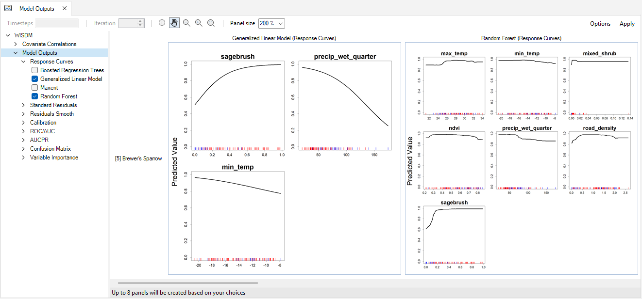
Under the Images tab, you will also find the Images Outputs tab. Outputs include Response Curves, Standard Residuals, Residuals Smooth, Calibration, ROC/AUC, AUCPR, Confusion Matrix, and Variable Importance. These outputs provide information on model performance and offer quick comparison of different statistical models.
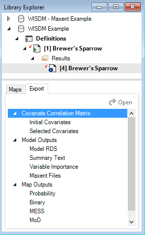
Export data
To export a map or model output created by the WISDM package, add the results scenario with the desired outputs to the results, then open the Export tab at the bottom of the screen. All available files for export will be listed. To export, simply double-click on the desired output and choose the directory in which to save the file in the pop-up window. Note that if multiple results scenarios are included in the active results scenarios, files for each of the selected scenarios will be exported.