⚠️ Notice to Users
The Getting Started documentation and associated Tutorials for this SyncroSim package currently reflects information for SyncroSim version 2. We are in the process of updating these pages to ensure compatibility with SyncroSim version 3. In the meantime, please note that some instructions, references, and/or images may not fully align with the latest version of SyncroSim. We appreciate your patience as we work to provide updated resources.
Reproducing the Omniscape.jl example with omniscape SyncroSim
This tutorial provides an overview of working with omniscape SyncroSim in the Windows user interface. It covers the following steps:
- Creating and configuring an omniscape SyncroSim Library
- Visualizing scenario results
- Creating, editing, and running a new scenario
- Comparing results across scenarios
Step 1. Creating and configuring an omniscape SyncroSim Library
In SyncroSim, a library is a file with extension .ssim that stores all the model’s inputs and outputs in a format specific to a given package. To create a new library:
1. Open SyncroSim Desktop.
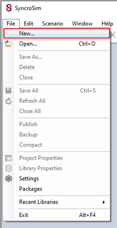
2. Select File > New.
b. Select the Omniscape Example template library. If desired, you may edit the File name, and change the Folder by clicking on the Browse button. Click OK.
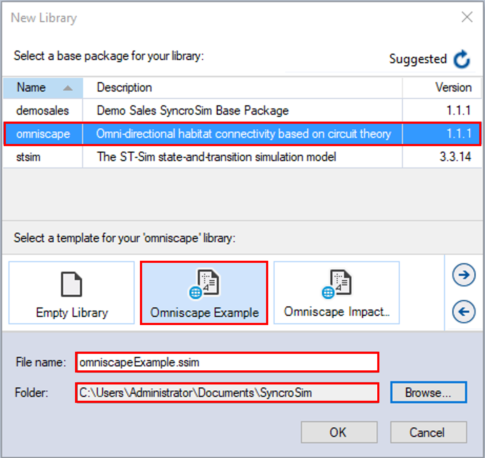
A new library has been created based on the selected template. SyncroSim will automatically open and display it in the Library Explorer window.
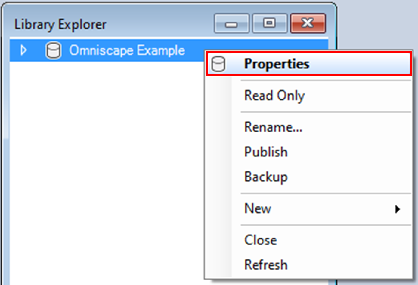
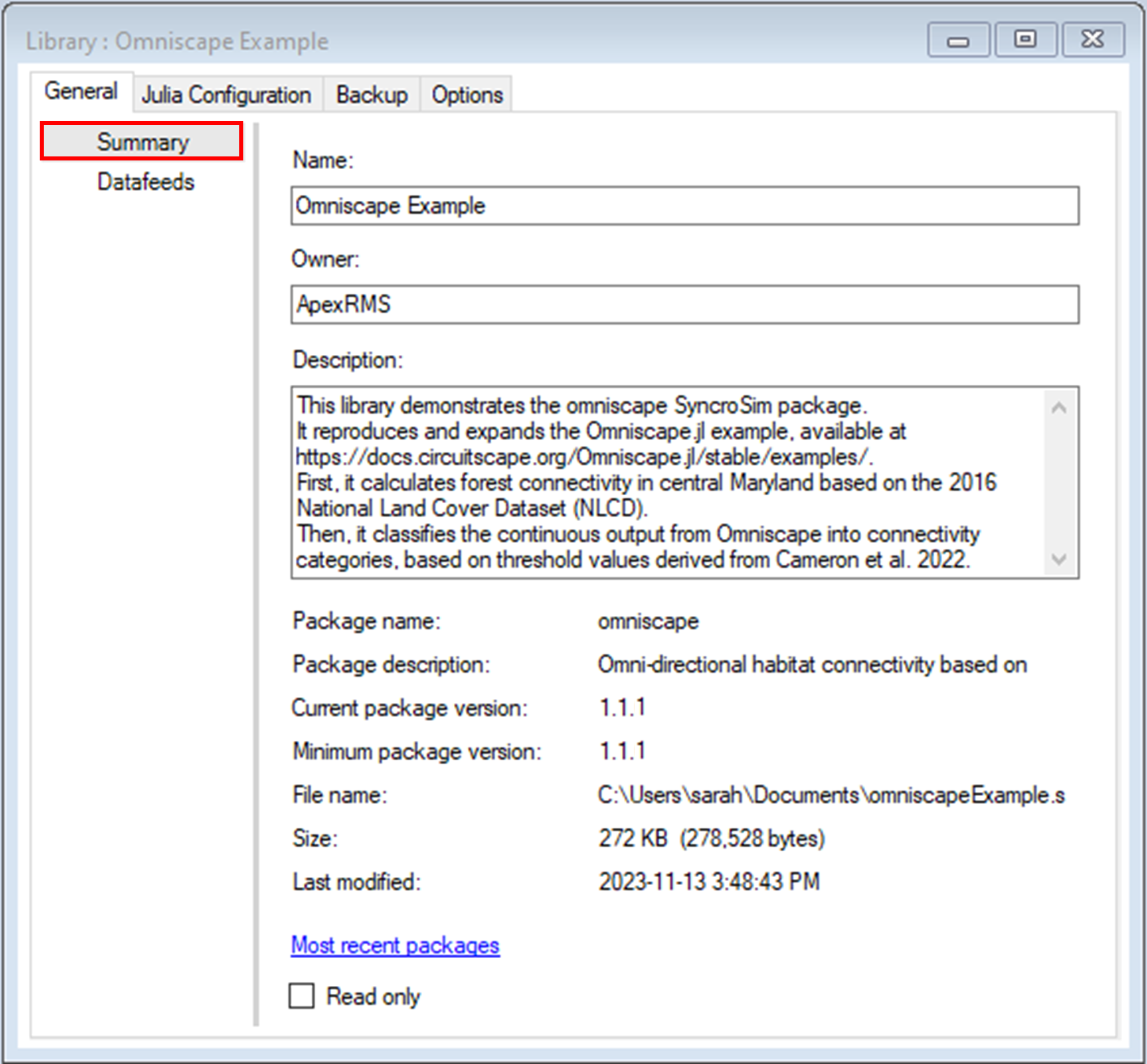
3. Double-click on the library name, Omniscape Example, to open the library properties window. You may also right-click on the library name and select Properties from the context menu.
4. The Summary datasheet contains the metadata for the library.
5. Navigate to the Julia Configuration tab.
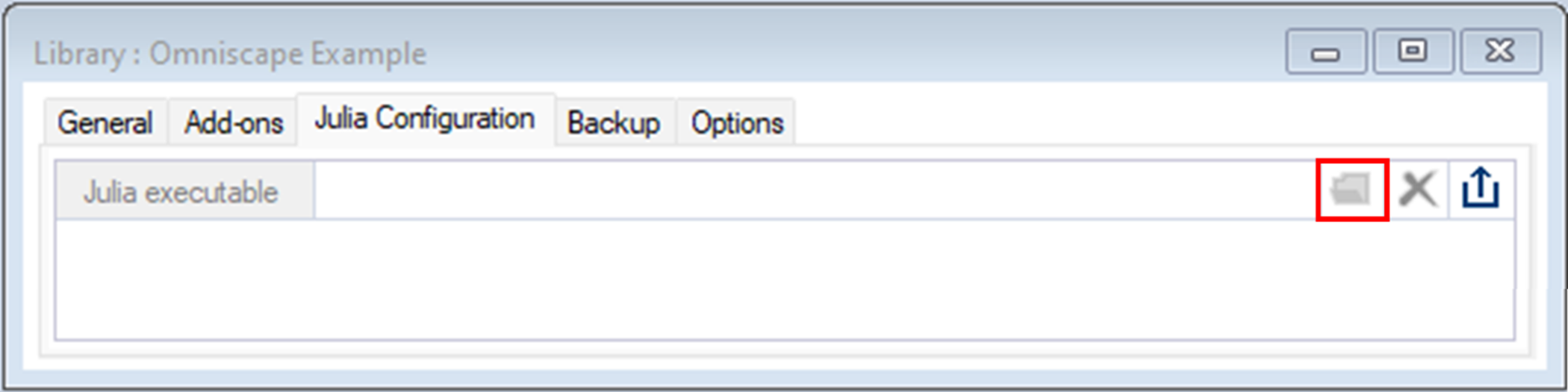
Note: The AppData folder is sometimes hidden. To see it, in File Explorer, select View > Show > Hidden items.
6. Next, navigate to the Options tab.
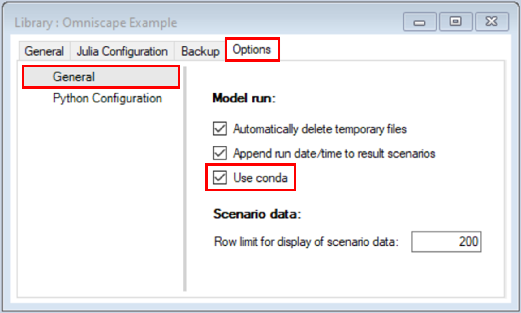
7. Close the library properties window.
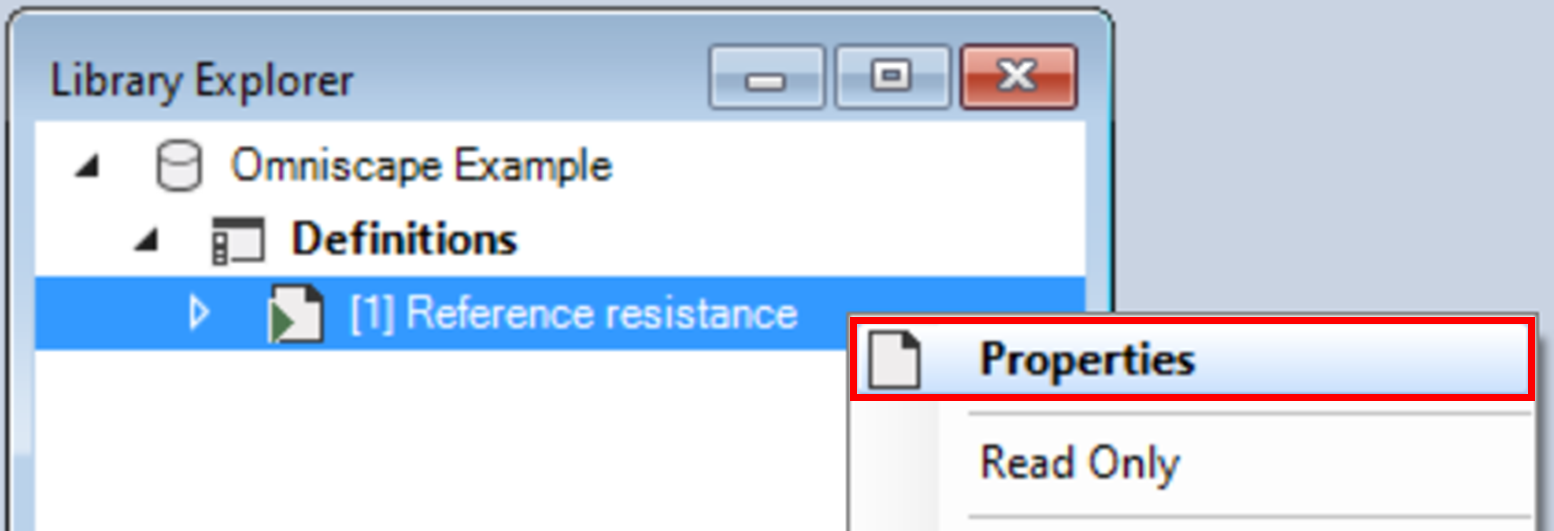
Next, you will review the inputs of the Reference resistance scenario. In SyncroSim, each scenario contains the model inputs and outputs associated with a model run.
1. In the Library Explorer window, select the pre-configured scenario Reference resistance and double-click it to open its properties. You may also right-click on the scenario name and select Properties from the context menu.
2. Navigate to the Pipeline datasheet.
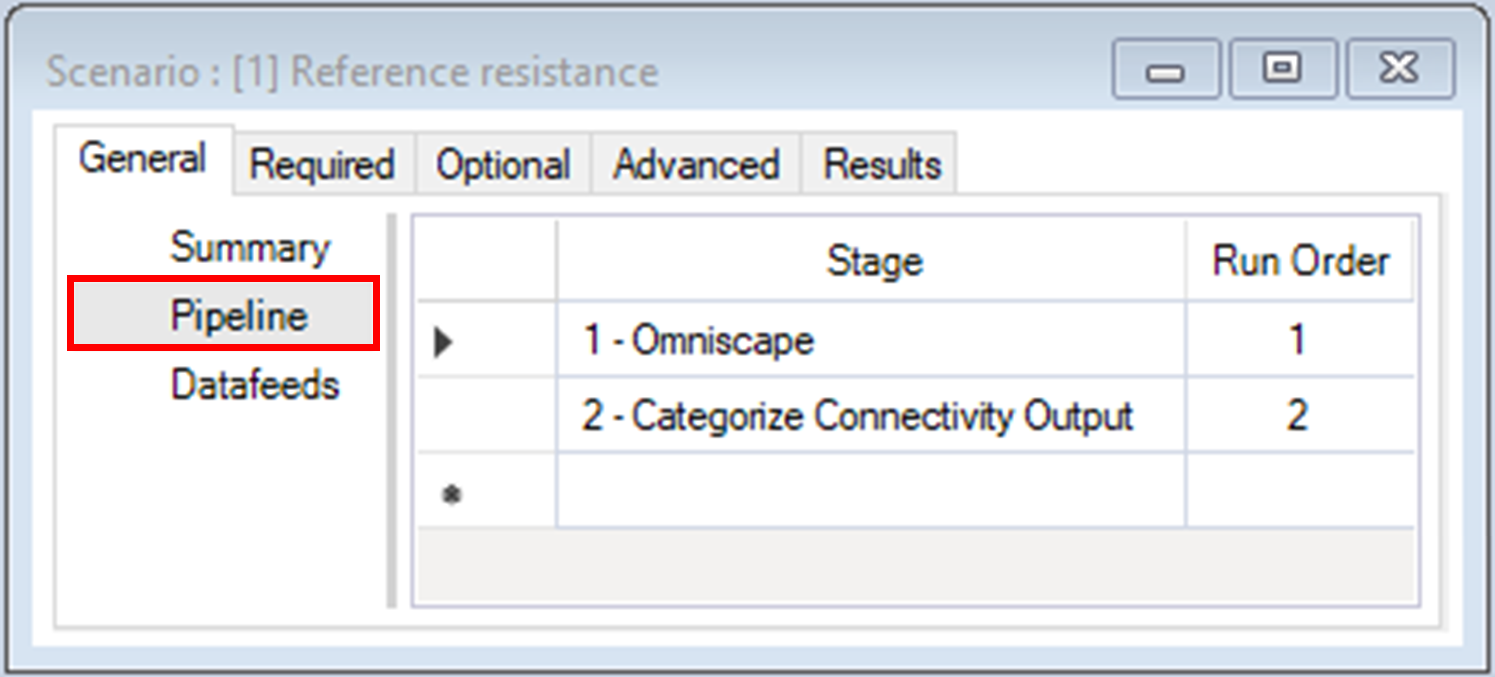
ii. Categorize Connectivity Output – classifies the continuous output from Omniscape.jl into connectivity categories based on a set of threshold values
The Omniscape pipeline stage replicates the exact structure and order of parameters as Omniscape.jl with inputs organized in two tabs: Required and Optional.
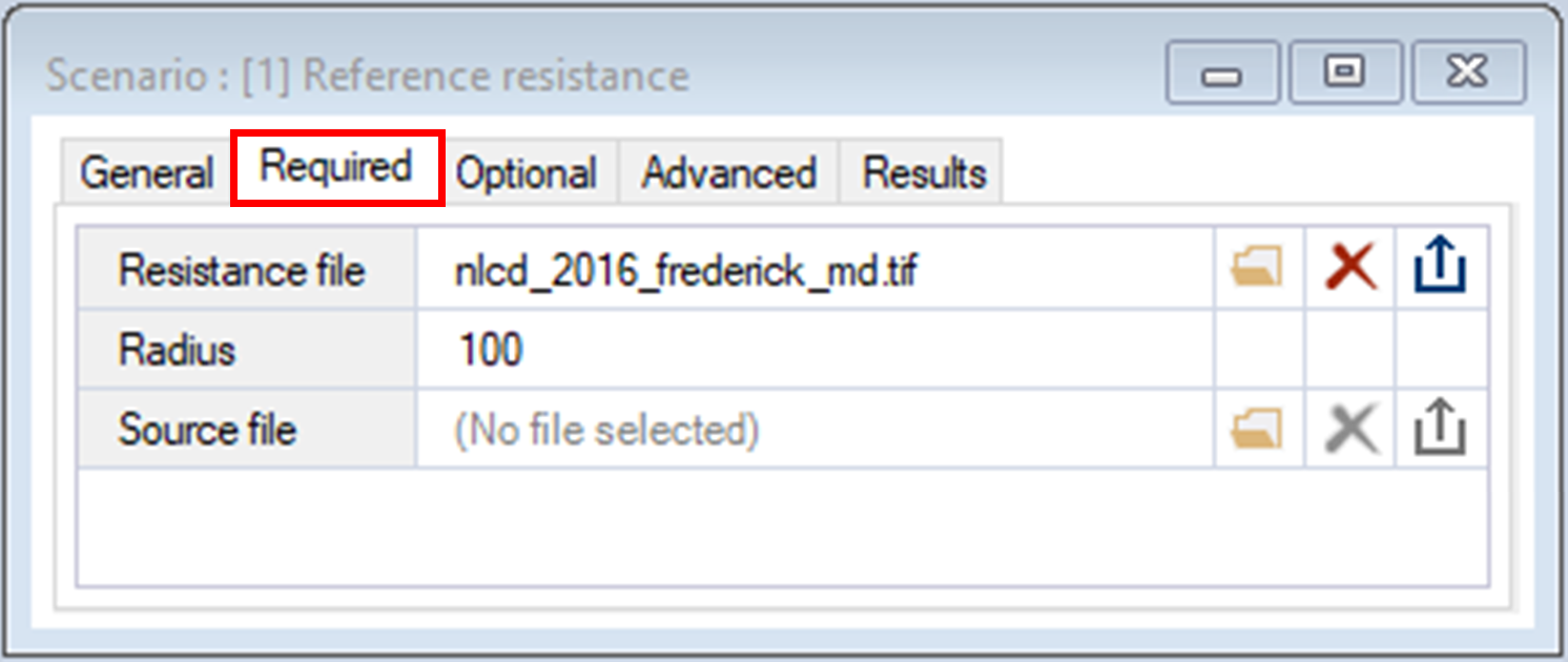
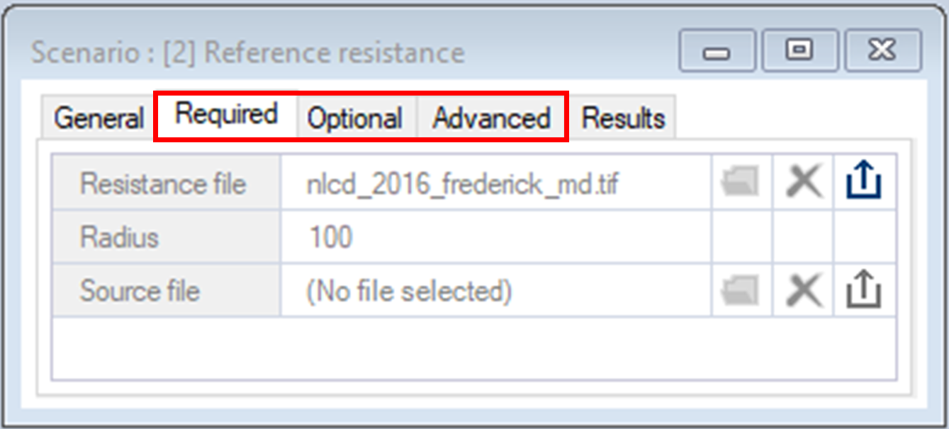
3. Navigate to the Required tab, which contains the following inputs:
b. Radius – sets the radius of the moving window. This example uses a radius of 100 pixels.
c. Source file – a raster file indicating which pixels correspond to sources. In this example, the sources are set through a different method, described in the next step.
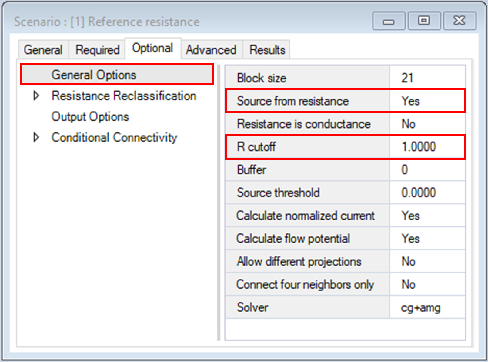
4. Navigate to the Optional tab.
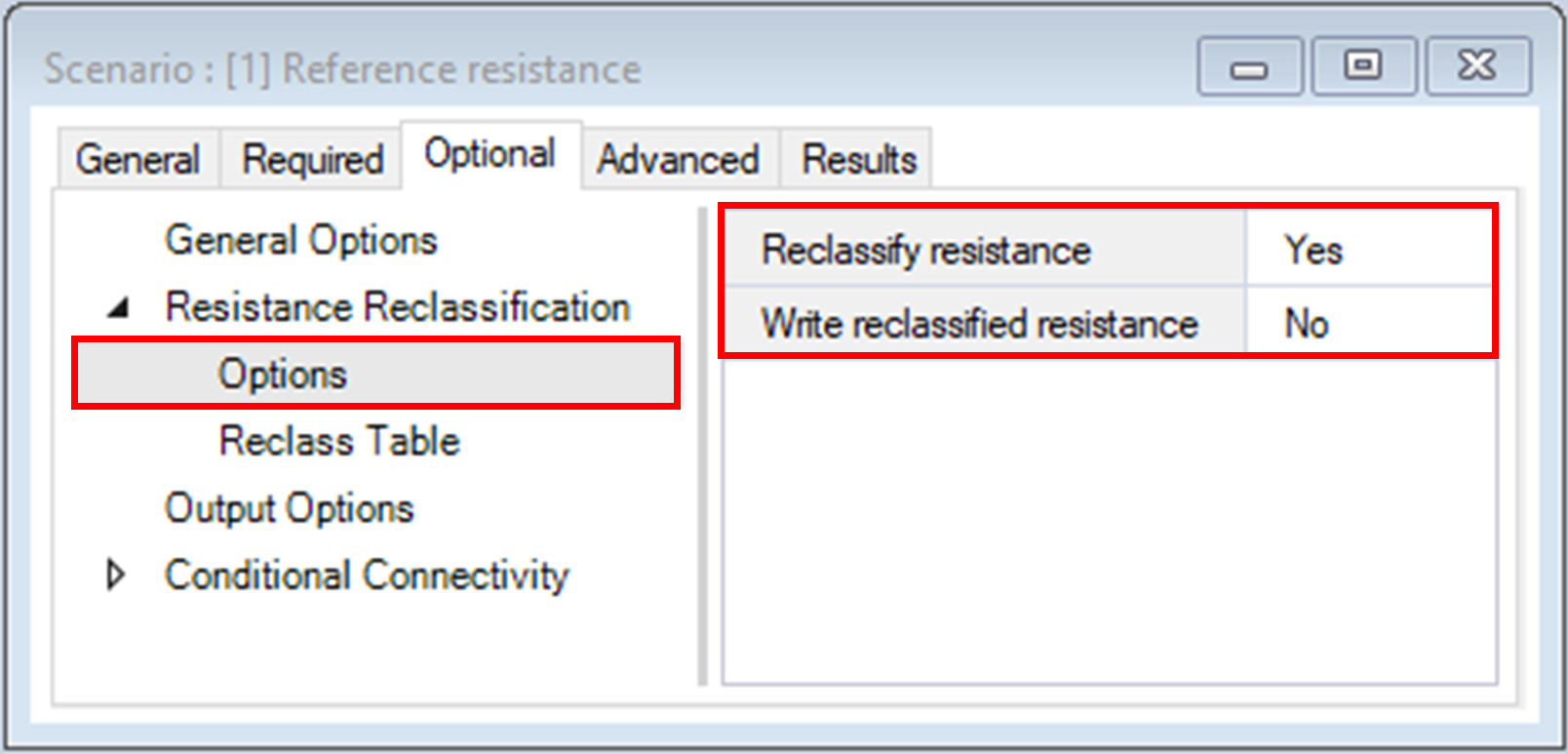
ii. Options > Write reclassified resistance – determines whether the reclassified resistance raster should be saved and written to file.
The Categorize Connectivity Output pipeline stage is an exclusive feature of the omniscape SyncroSim package. It allows for seamless post-processing of the continuous output of Omniscape into discrete connectivity categories based on user-defined connectivity categories, a common step in the Omniscape workflow.
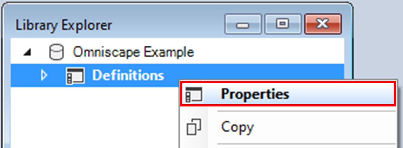
5. In the Library Explorer, double-click on Definitions to open the project properties. You may also right-click on the project name and select Properties from the context menu.
6. Under the Summary datasheet, the Description field highlights that the connectivity categories and thresholds used in the template library were derived from Cameron et al. (2022, Conservation Science and Practice).
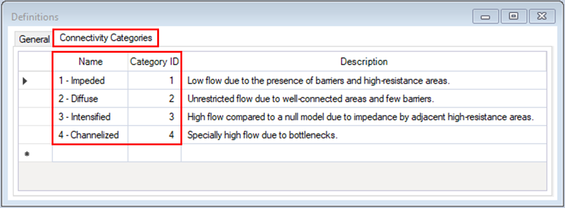
7. Navigate to the Connectivity Categories tab.
b. Click on the Category ID column to sort categories in ascending order, where Impeded represents areas with the least amount of flow, and Channelized represents areas with the greatest amount to flow.
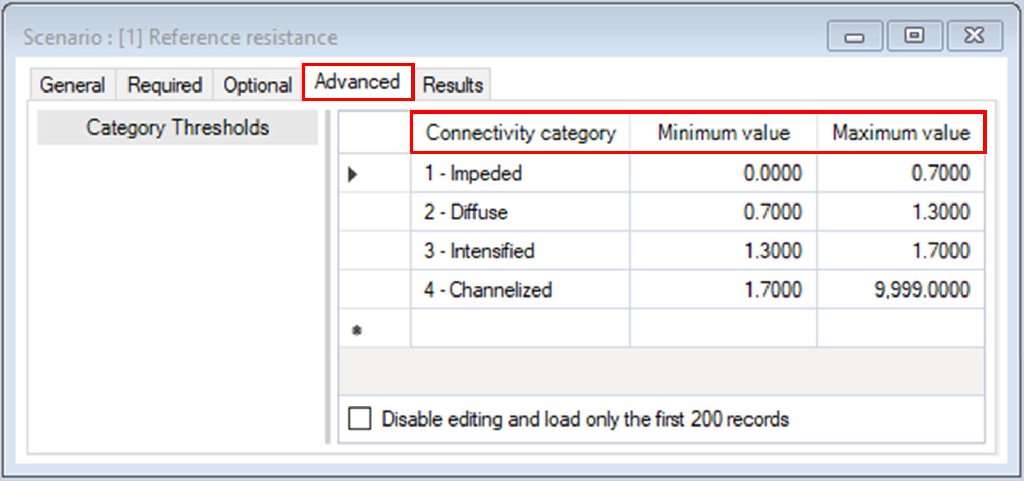
8. Return to the scenario properties window, navigate to the Advanced tab.
9. Close the scenario properties window.
Step 2. Visualizing scenario results
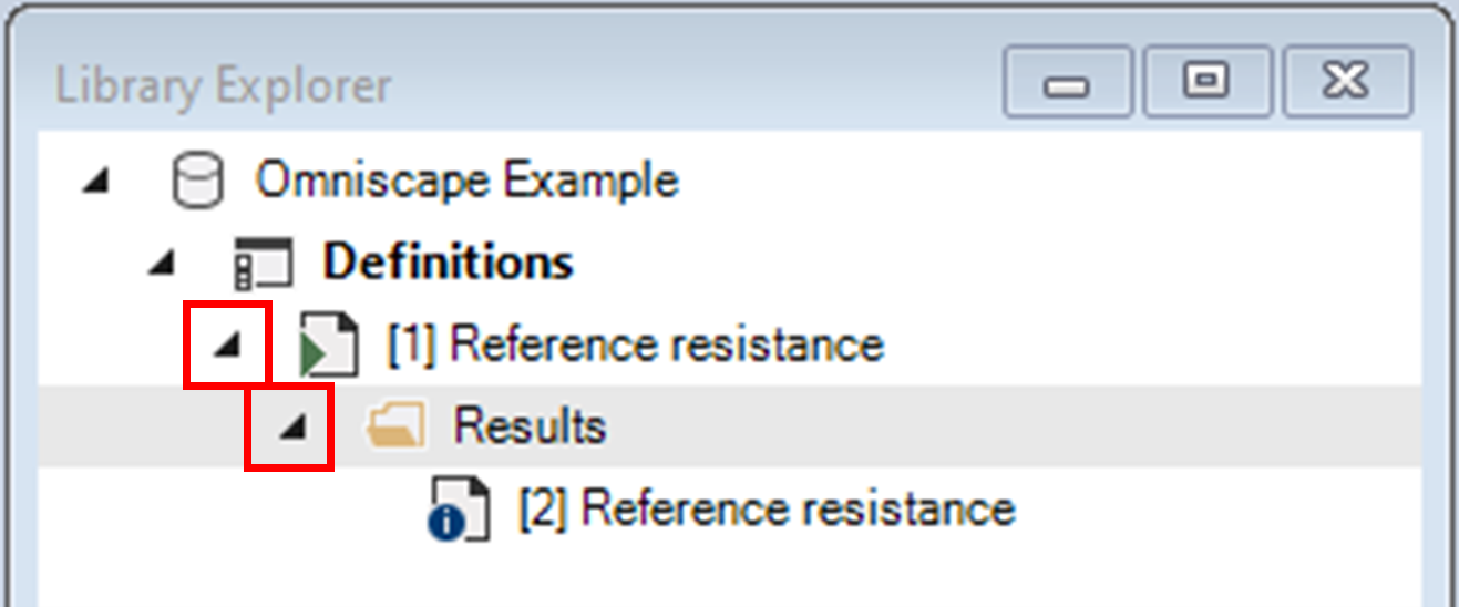
The Omniscape Example template library already contains the results for the Reference resistance scenario. In SyncroSim, the results for a scenario are organized into a Results folder, nested within its parent scenario.
1. In the Library Explorer window, click on the arrow beside the Reference resistance scenario to expose the Results folder; repeat the same action to expose the results scenario.
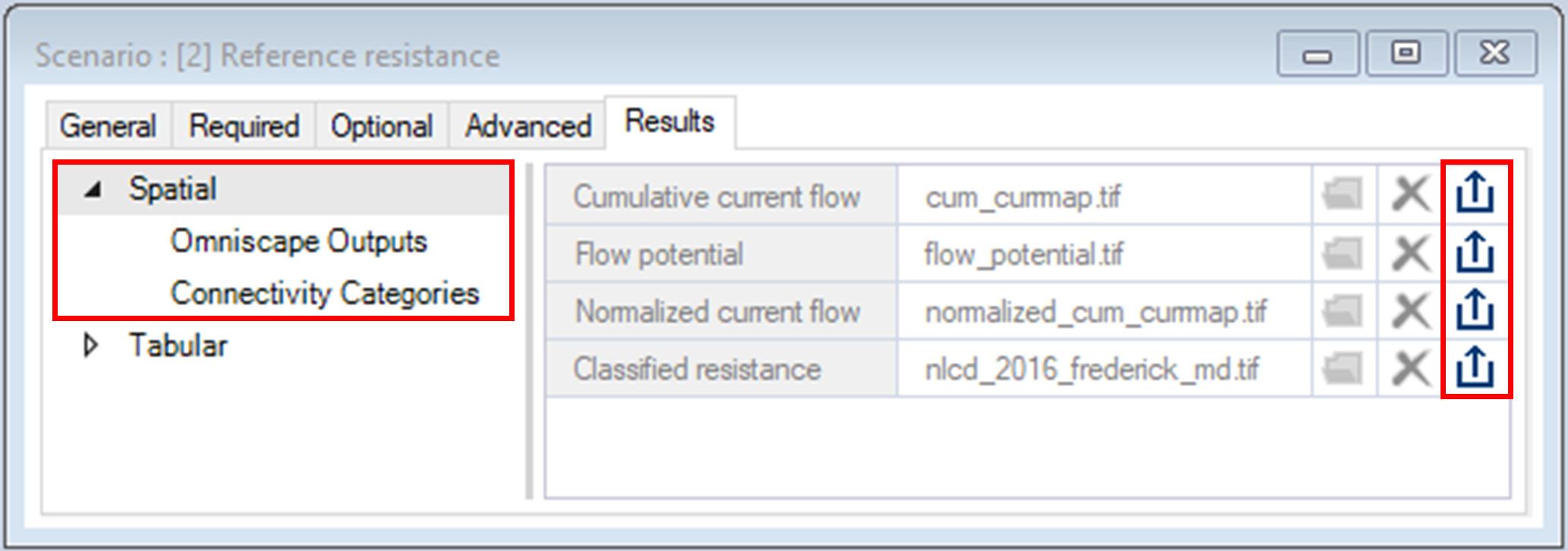
2. Double-click on the results scenario to open its properties.
You can export any spatial output by clicking on the Export button.
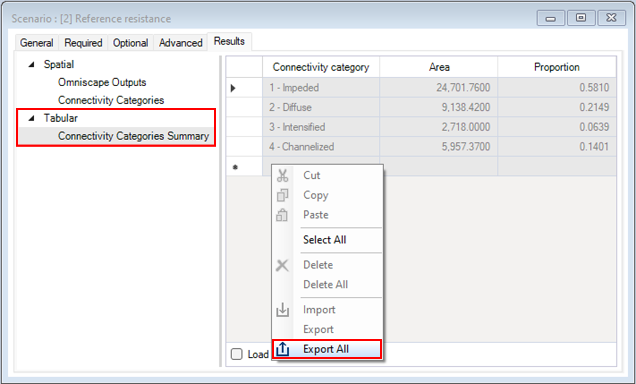
You can export the tabular output by right-clicking on the data and selecting Export All from the context menu.
3. Close the results scenario properties.
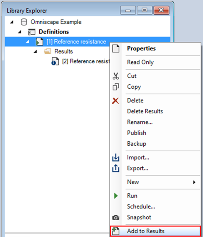
4. In the Library Explorer window, right-click on the Reference resistance scenario and select Add to Results from the context menu.
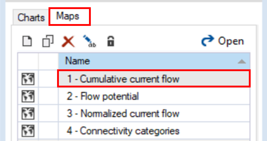
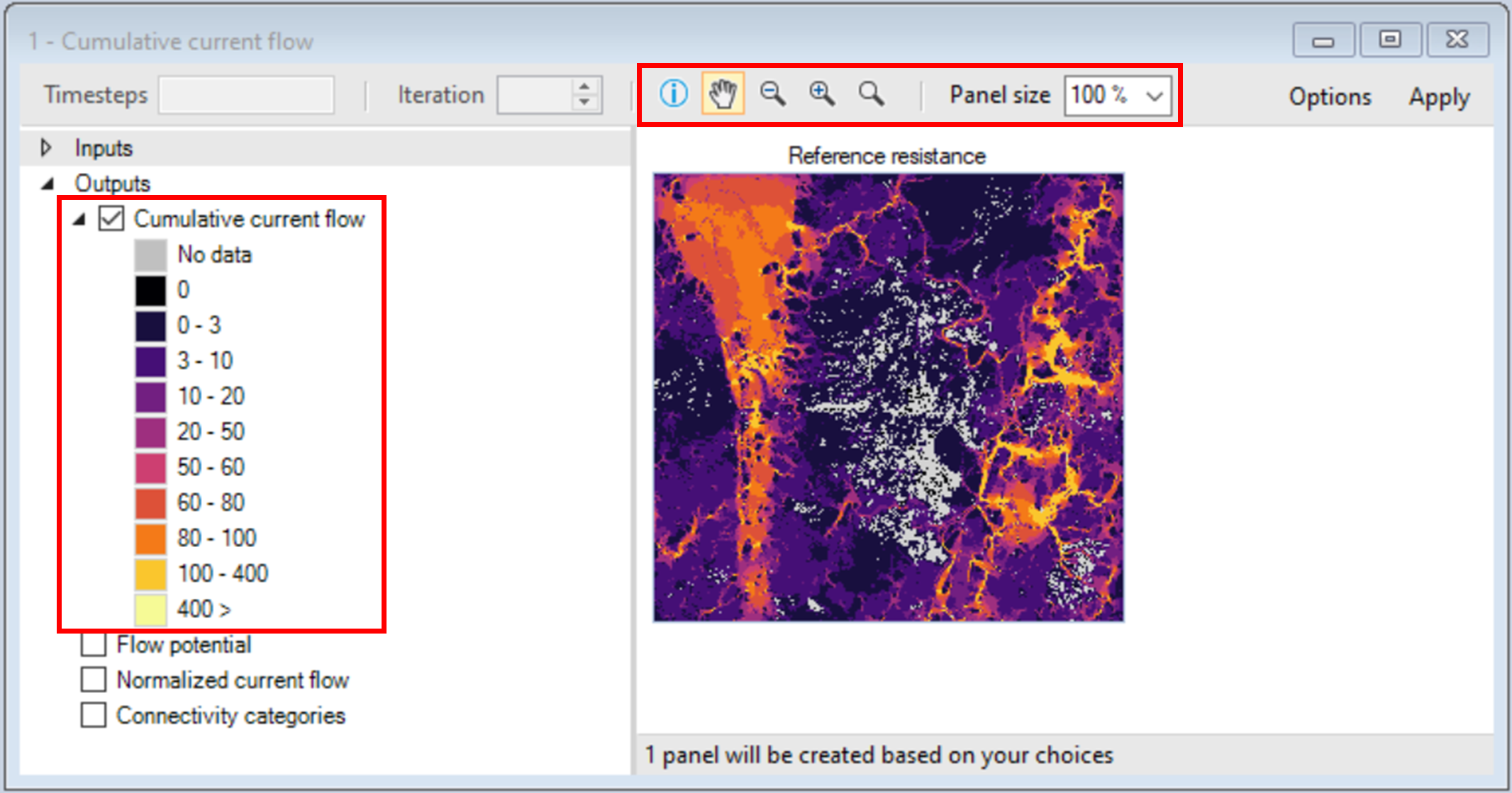
5. Navigate to the Maps tab and double-click on the first pre-configured map, Cumulative current flow.
b. Toolbar – displayed along the top of the window. Includes zoom, pan and per pixel information tooltip.
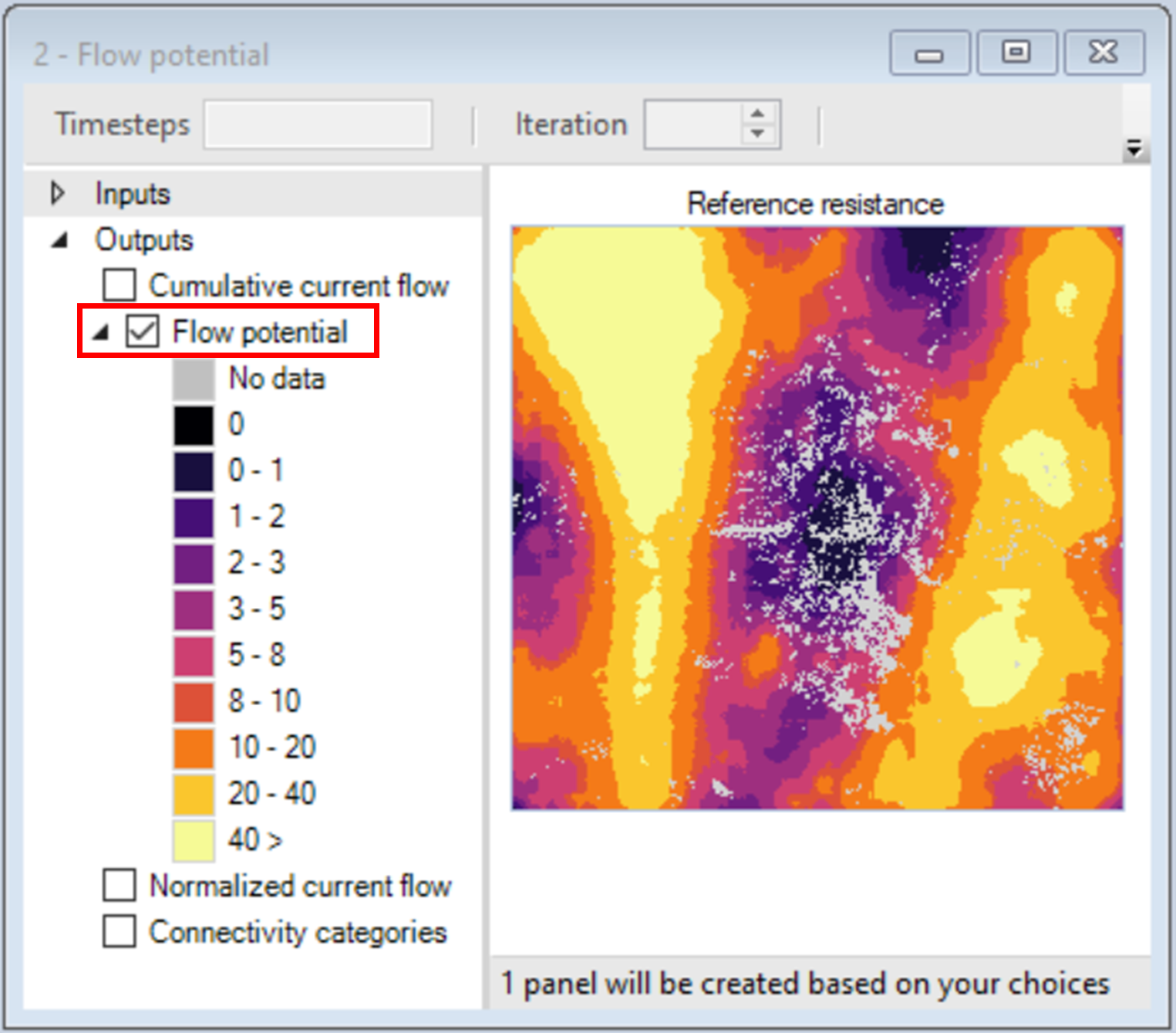
6. Close the map window and view the two following maps.
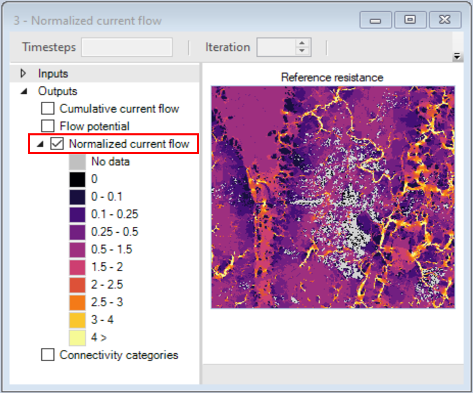
Next, you will visualize the outputs of the second transformer, which takes the Normalized current flow map and reclassifies it into a discrete map, based on the threshold values reviewed in steps 13-17.
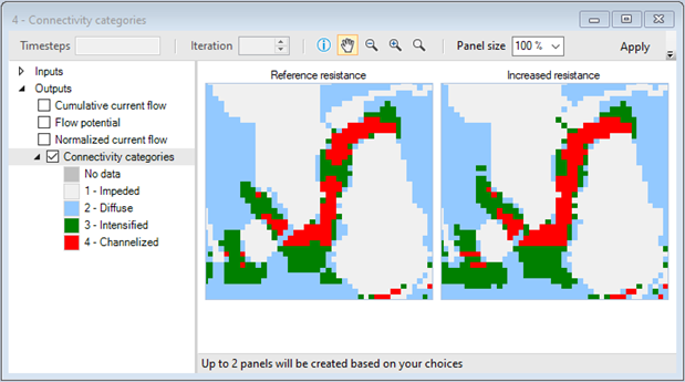
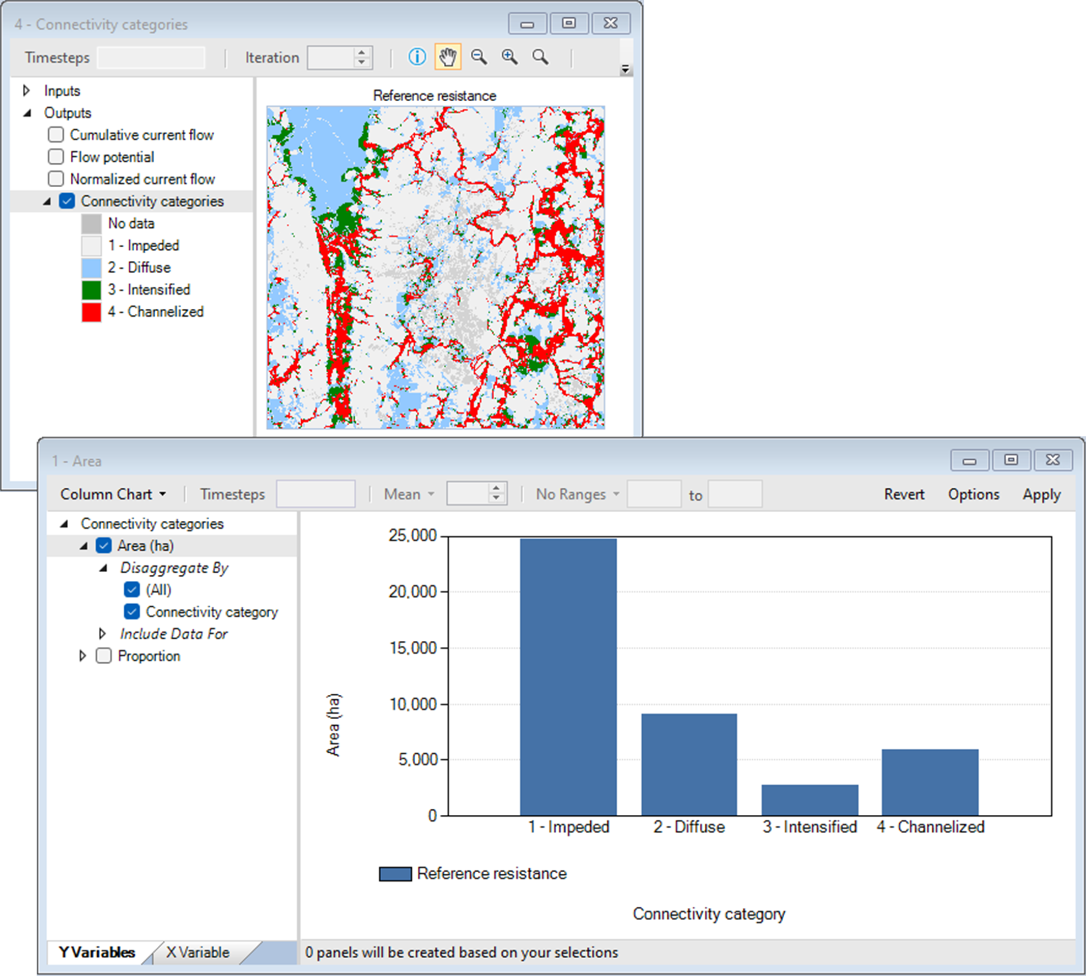
7. View the Connectivity categories map.
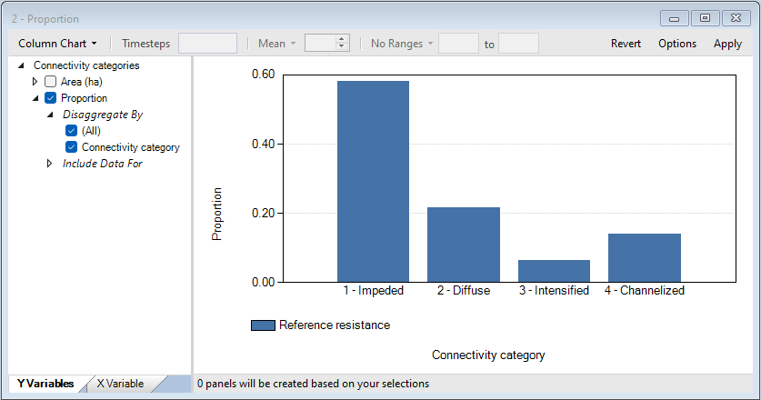
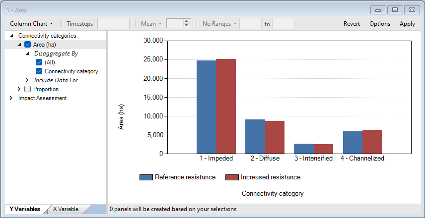
8. Keep the map open for comparison and from the Library Explorer window, navigate to the Charts tab and view the Area chart.
9. Close all plot windows.
Step 3. Creating, editing, and running a new scenario
Next, you will learn how to create a scenario and run it to generate results. This scenario will differ from the Reference resistance by a ten-fold increase in resistance for all non-forest (i.e., non-source) pixels.
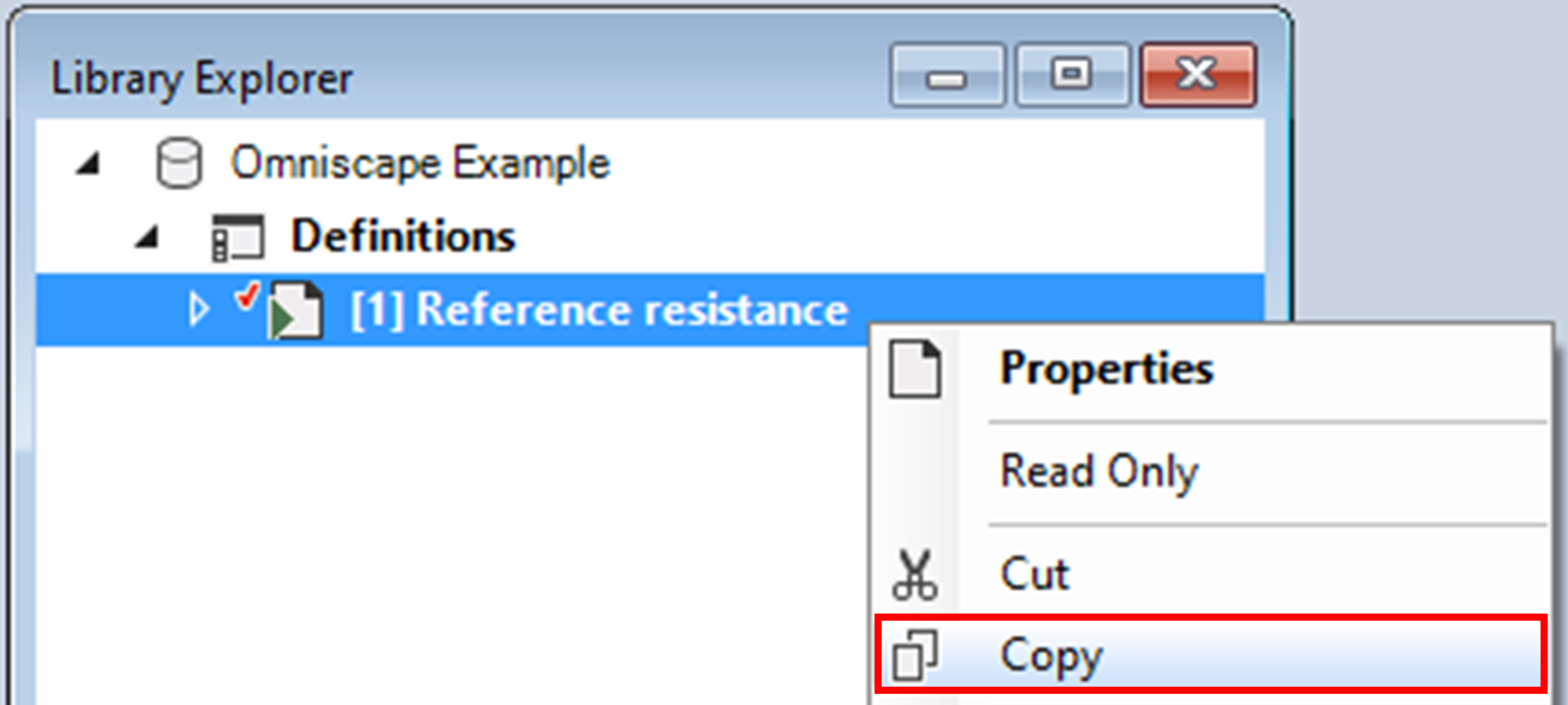
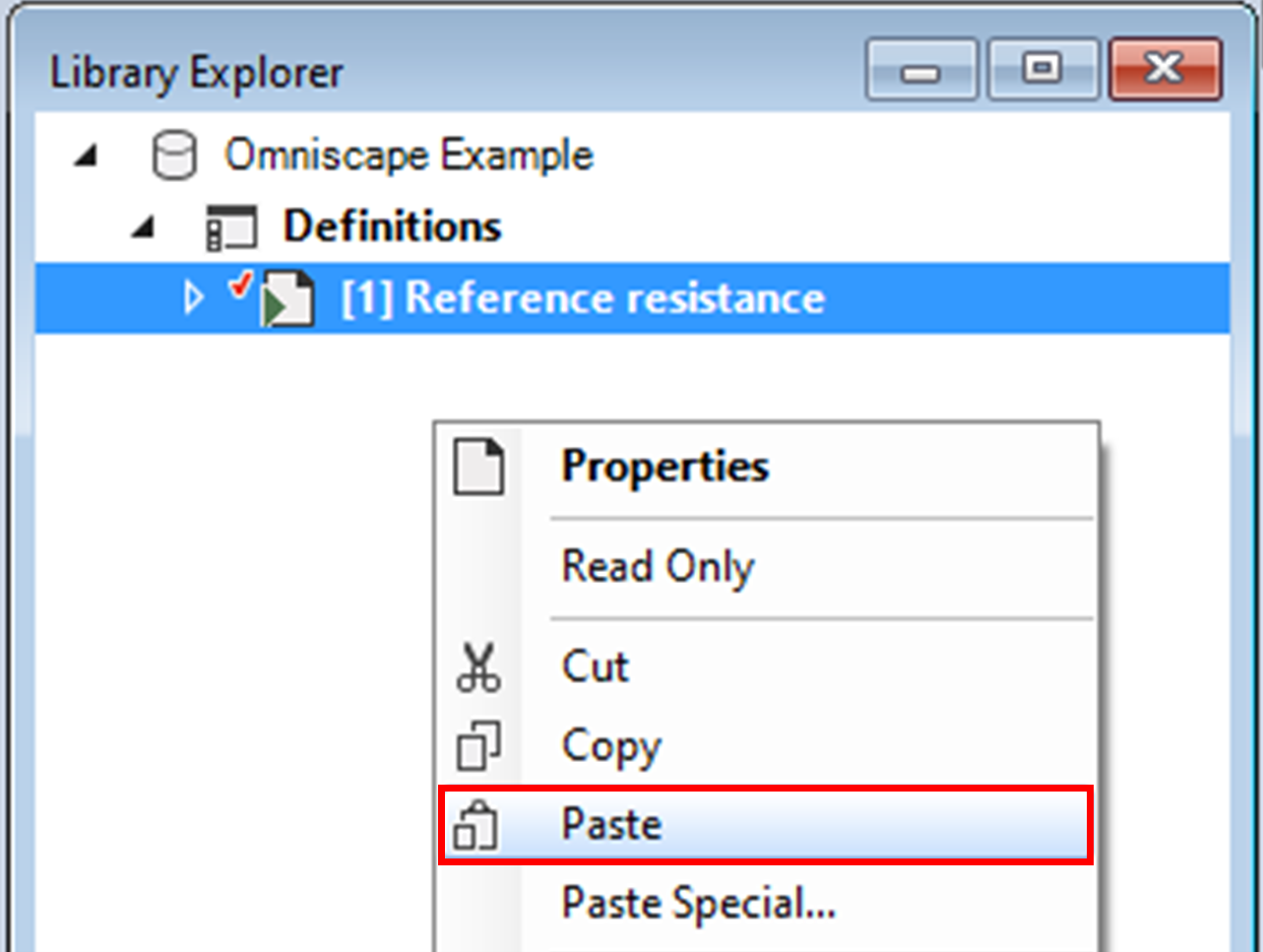
1. Right-click on the existing scenario and select Copy from the context menu.
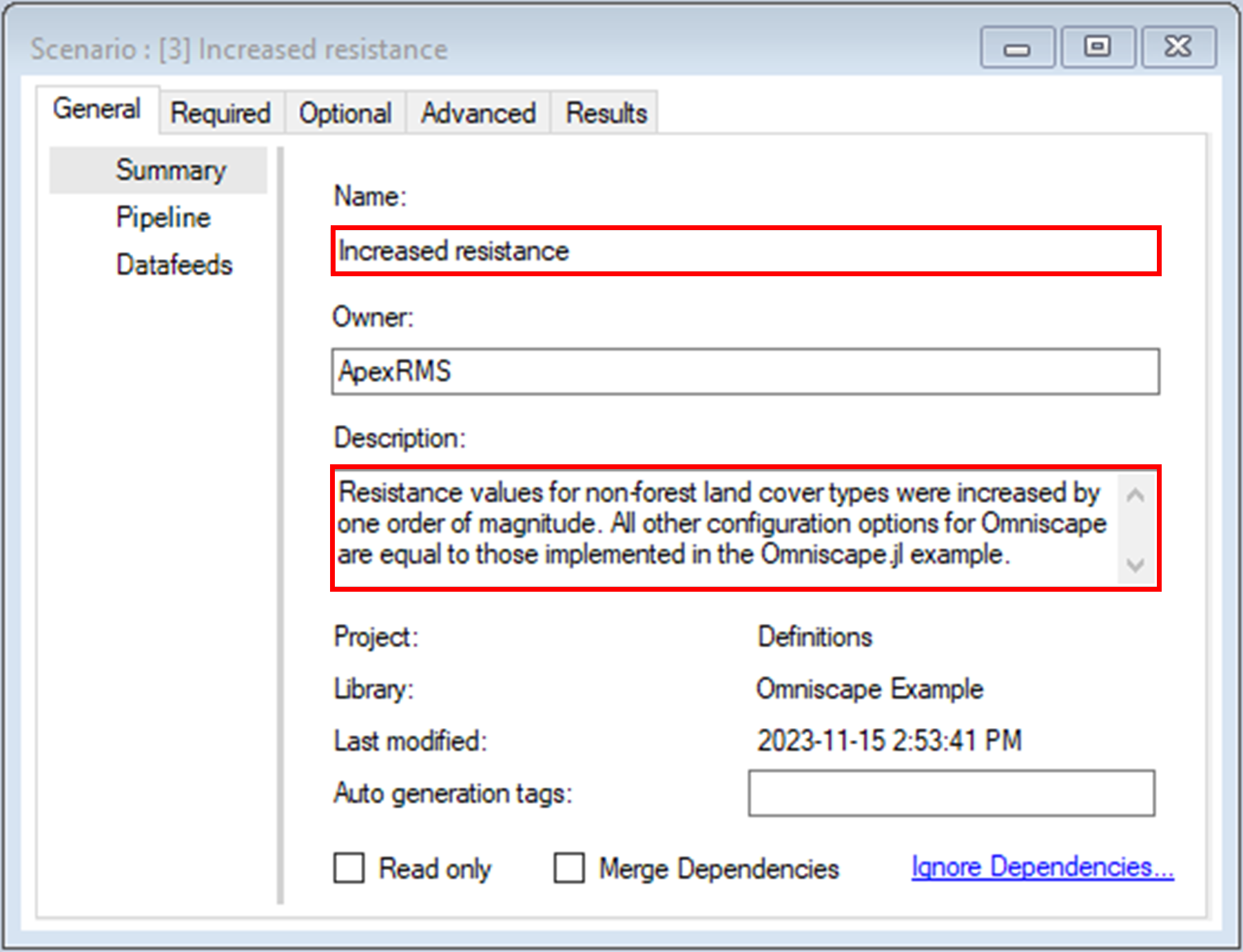
2. Double-click on the new scenario to open its properties.
b. Change the Description to Resistance values for non-forest land cover types were increased by one order of magnitude. All other configuration options for Omniscape are equal to those implemented in the Omniscape.jl example.
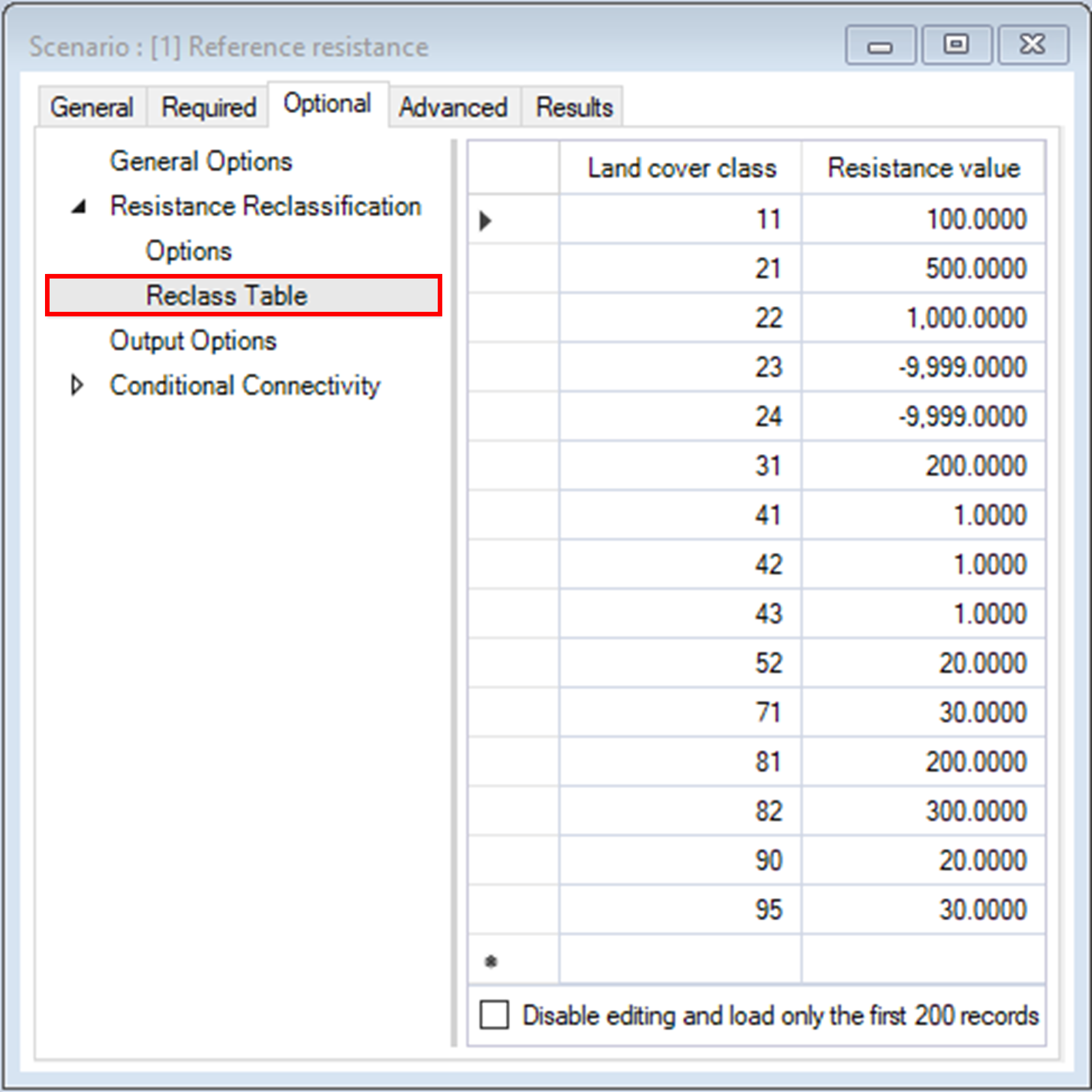
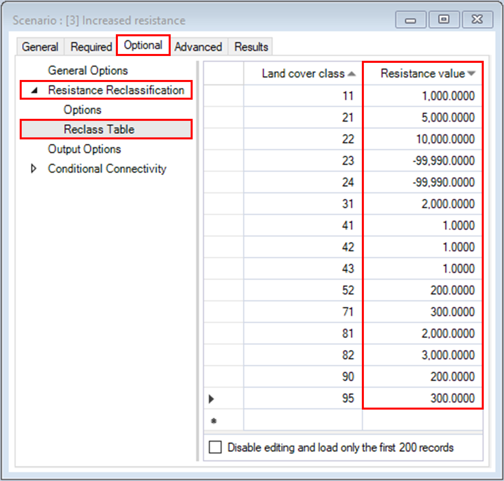
3. Navigate to the Optional tab and under the Resistance Reclassification node, open the Reclass table datasheet.
4. Close the scenario properties window and save the changes to the library.
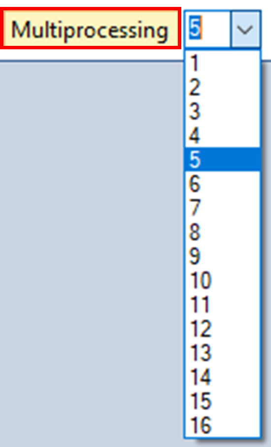
Next, you will run the scenario. For this example, the run should take approximately 10 minutes with multiprocessing enabled across 5 cores.
5. To enable multiprocessing, click on the Multiprocessing button along the SyncroSim toolbar and adjust the number of Multiprocessing jobs to 5.
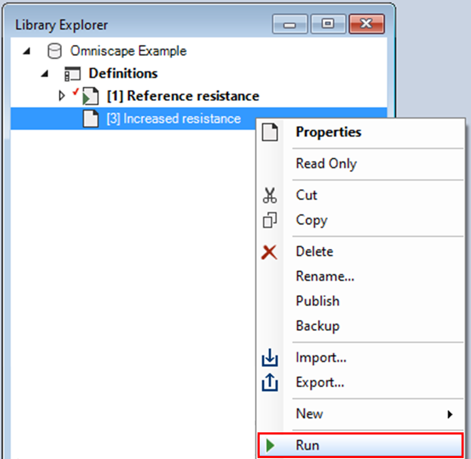
6. In the Library Explorer window, right-click on the Increased resistance scenario and select Run for the context menu.
c. First, SyncroSim calls the first transformer, Omniscape.
ii. Running Omniscape – the transformer calls Julia to run the analysis. Once the analysis is complete, the transformer retrieves and saves the outputs back to SyncroSim.
ii. Categorizing connectivity output – the transformer reclassifies the continuous output and returns it back to SyncroSim.
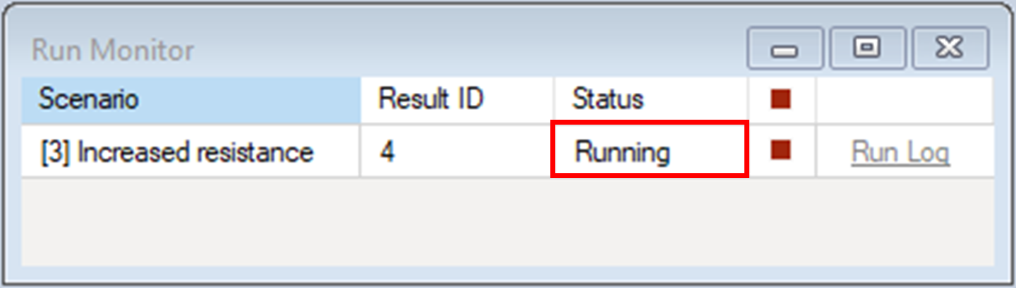
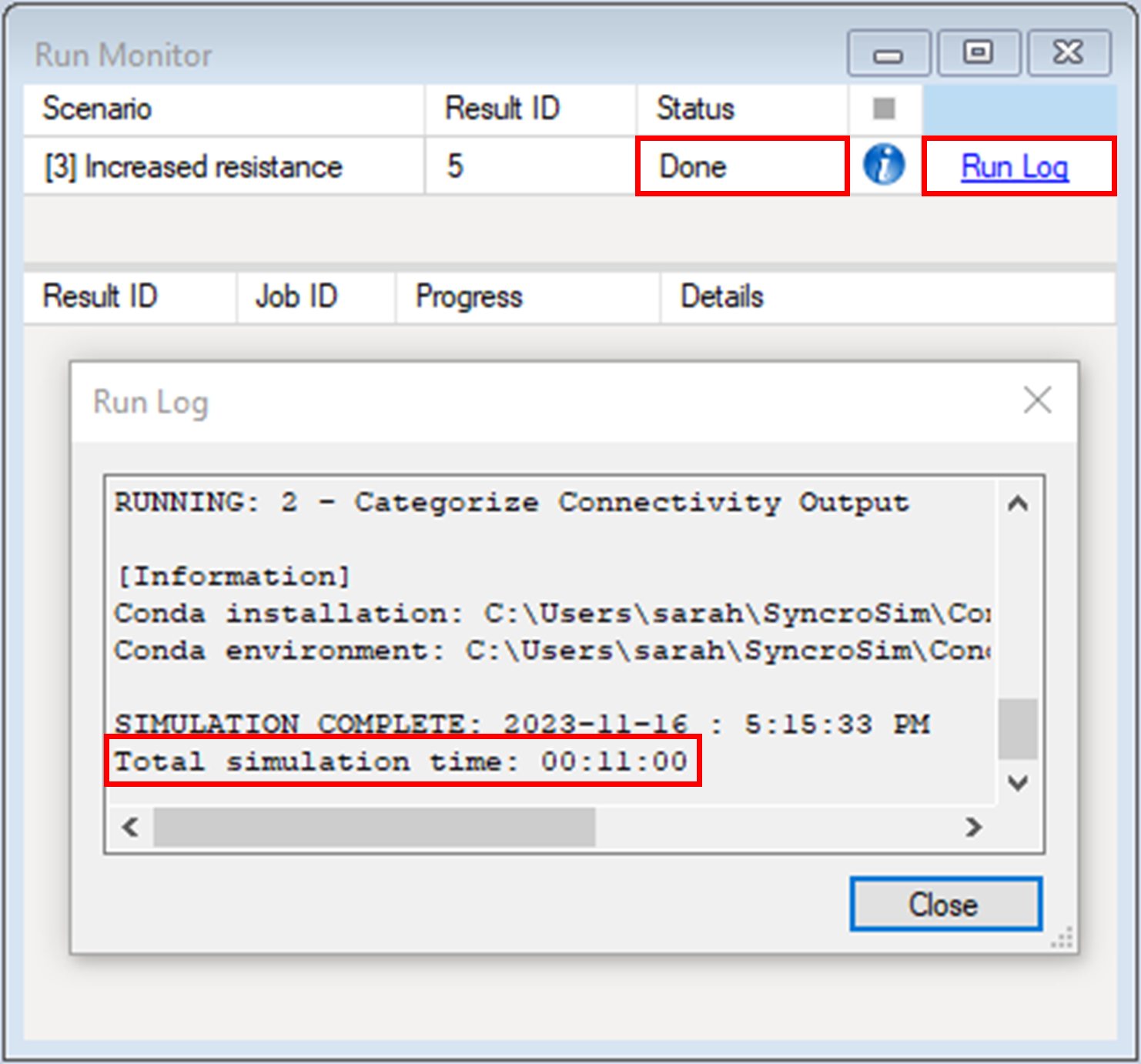
7. When the run is complete, the Status will be updated to Done. You can inspect the Run Log, which returns the total run time for the scenario.
Step 4. Comparing results across scenarios
With two successful scenario runs, you will now compare their results.
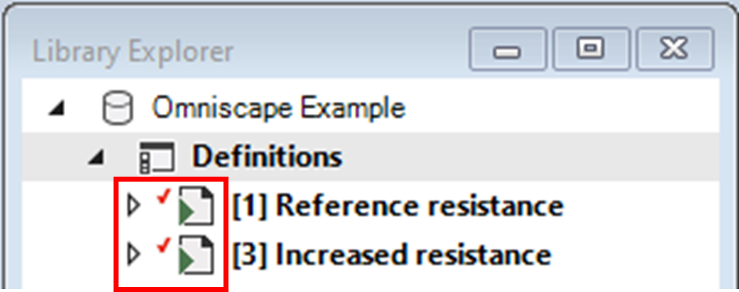
1. Ensure that both scenarios are added to the results. This is noted by a red check mark beside the scenario symbol and a bolded scenario name.
2. First, view the Area chart.
3. Next, view the Connectivity categories map.