⚠️ Notice to Users
The Getting Started documentation and associated Tutorials for this SyncroSim package currently reflects information for SyncroSim version 2. We are in the process of updating these pages to ensure compatibility with SyncroSim version 3. In the meantime, please note that some instructions, references, and/or images may not fully align with the latest version of SyncroSim. We appreciate your patience as we work to provide updated resources.
Measuring the impact of connectivity change with omniscapeImpact
This tutorial guides you through using the omniscapeImpact add-on package to omniscape SyncroSim. It covers the following steps:
- Installing the omniscapeImpact package
- Creating and configuring an omniscapeImpact SyncroSim Library
- Visualizing and comparing scenario results
Requirements
Before you begin, make sure that the omniscape SyncroSim package version 1.1.1 is installed. For more information, see Installing the omniscape SyncroSim package.
Step 1. Installing the omniscapeImpact package
1. Open SyncroSim Desktop.
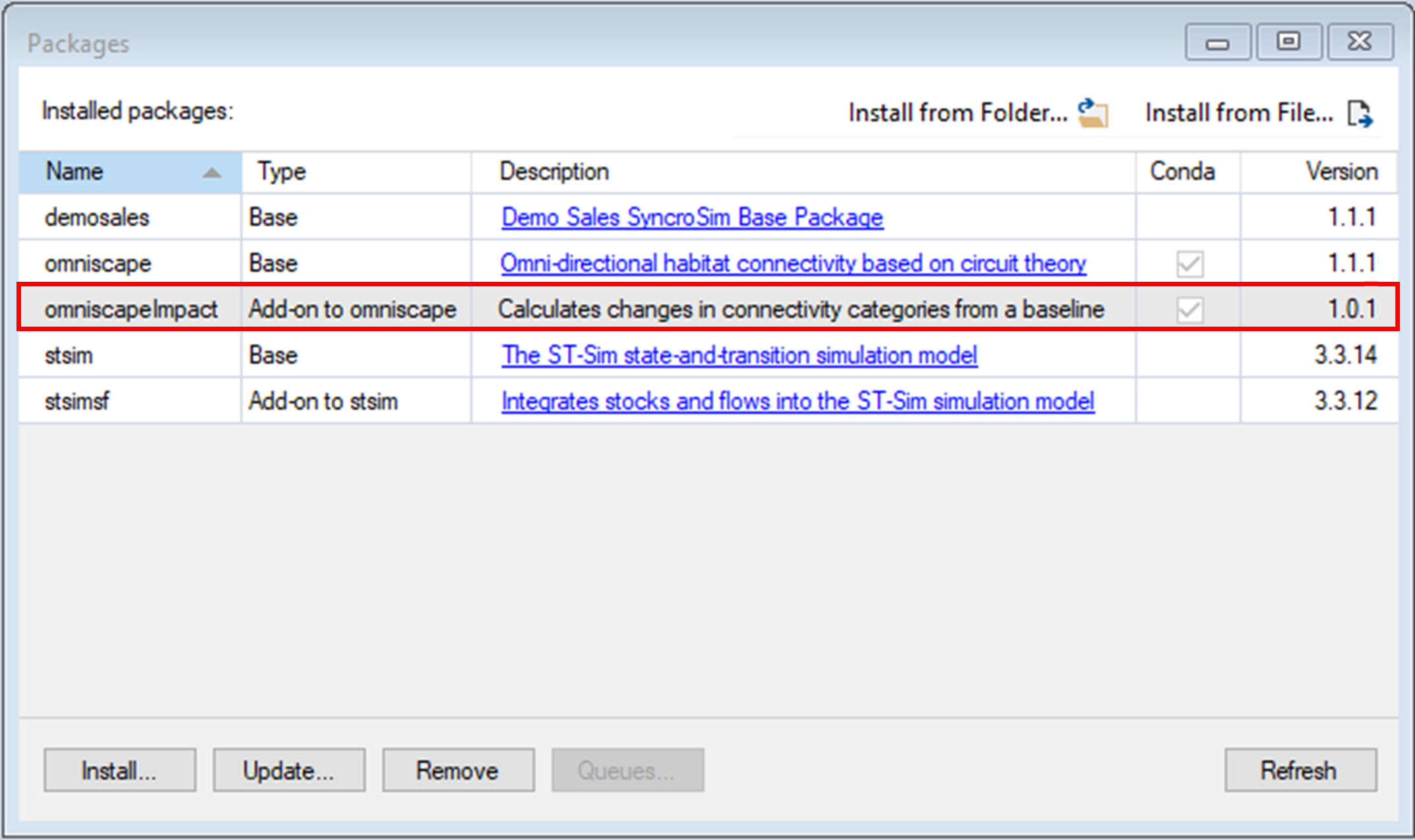
2. Select File > Packages.
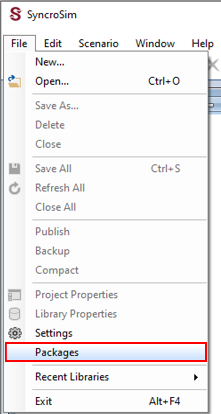
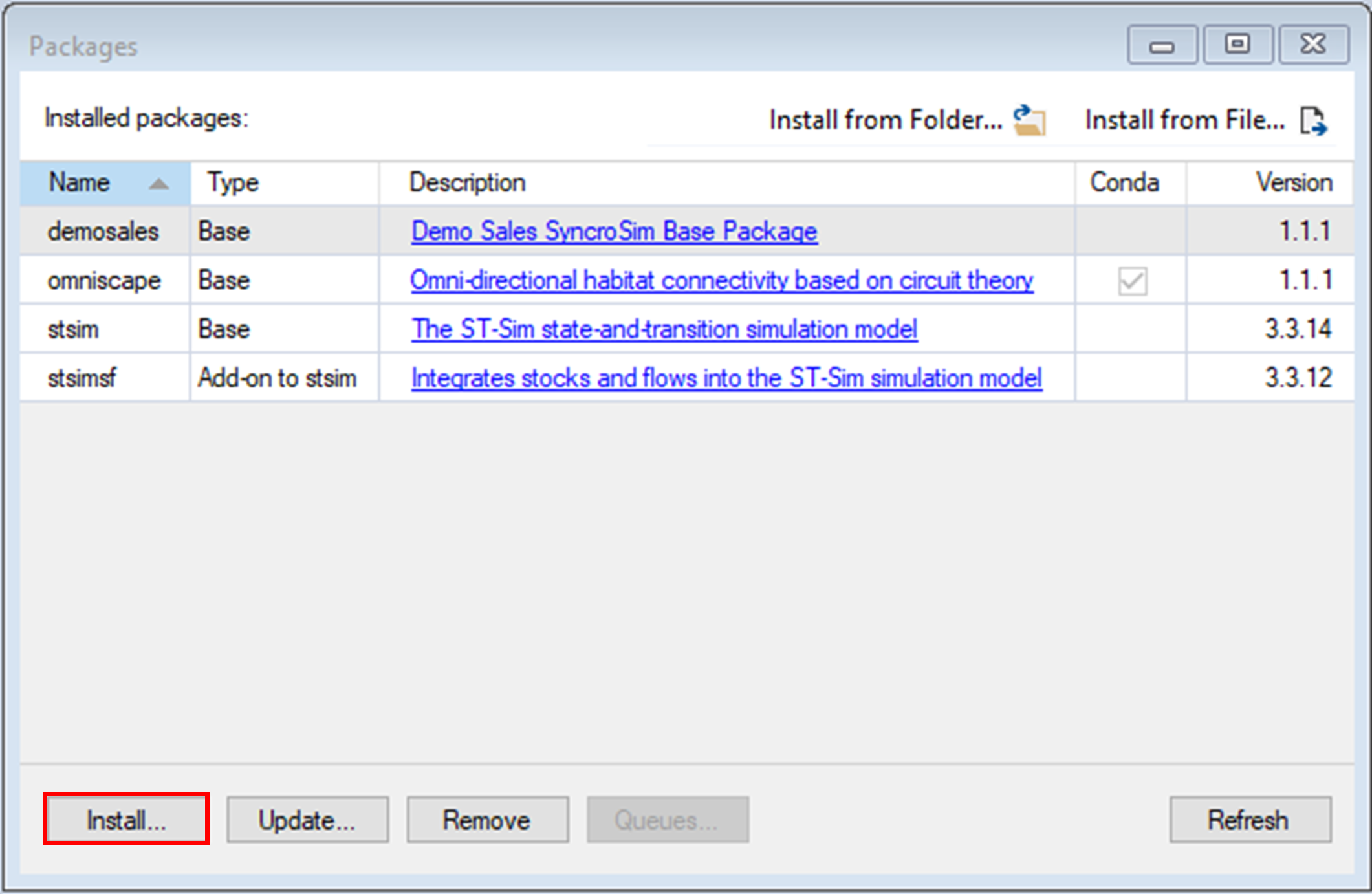
3. The Packages window will open, listing all the SyncroSim packages installed in your computer. To install a new package from the Package Server, click Install.
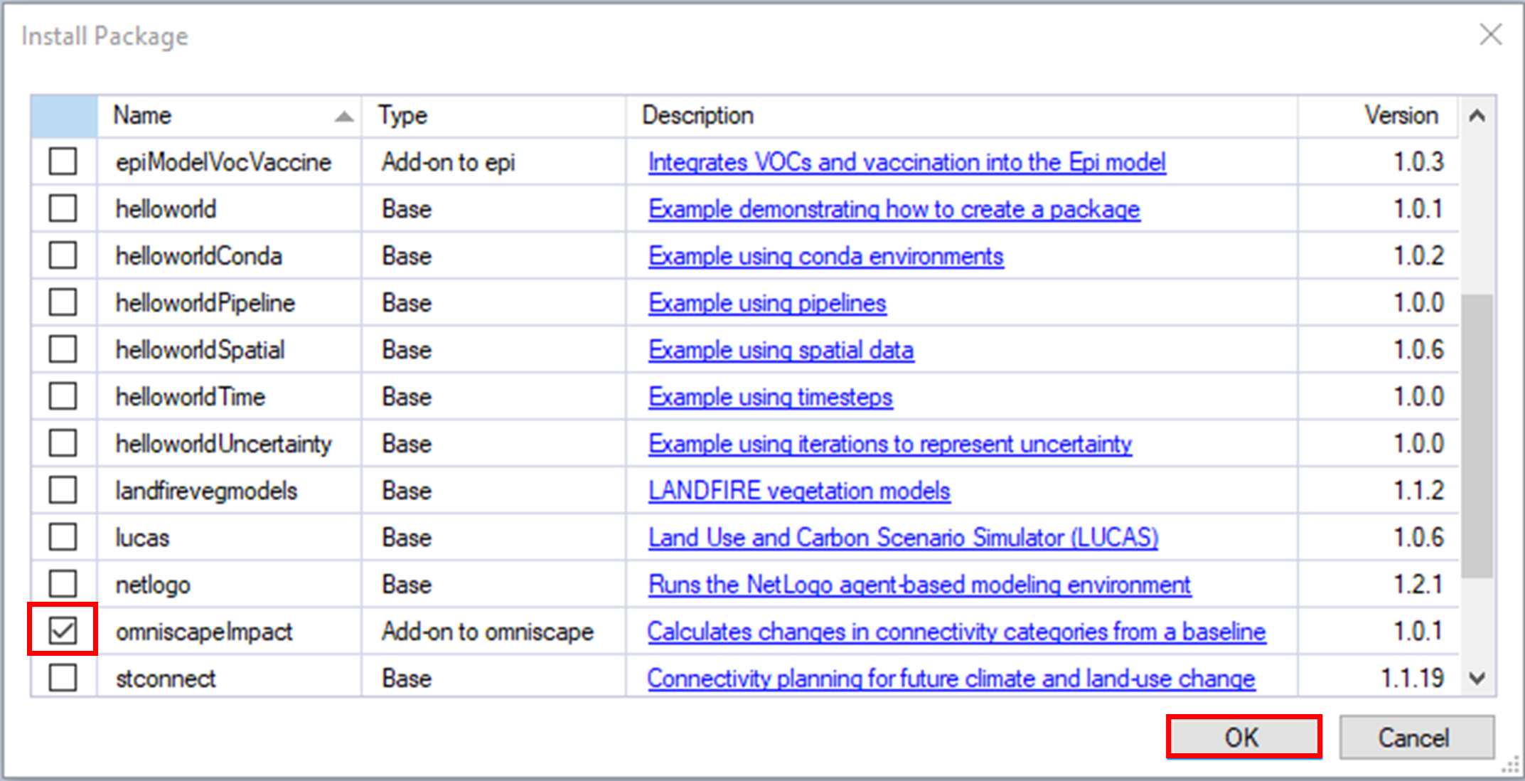
4. A new window will open listing the packages available for install from the Package Server. To install omniscapeImpact, mark the checkbox beside the package name and click OK.
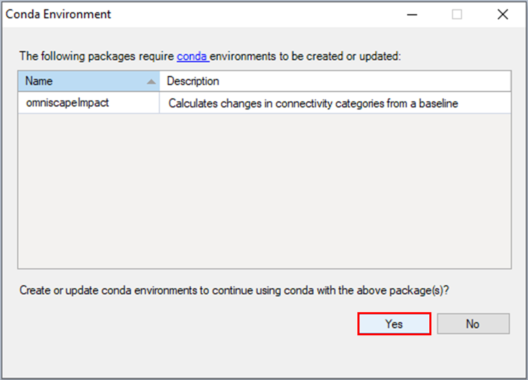
5. The omniscapeImpact package uses Conda to manage the package dependencies. Upon installing the package, you will be prompted to create or update the Conda environment for omniscapeImpact. Click Yes.
6. Return to the Packages window. omniscapeImpact will now be listed along with the other installed packages, and the Conda checkbox will be marked.
Step 2. Creating and configuring an omniscapeImpact SyncroSim Library
1. Open SyncroSim Desktop.
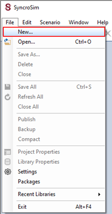
2. To create a new library, select File > New.
b. Select the Omniscape Impact template library. If desired, you may edit the File name, and change the Folder by clicking on the Browse button. Click OK.
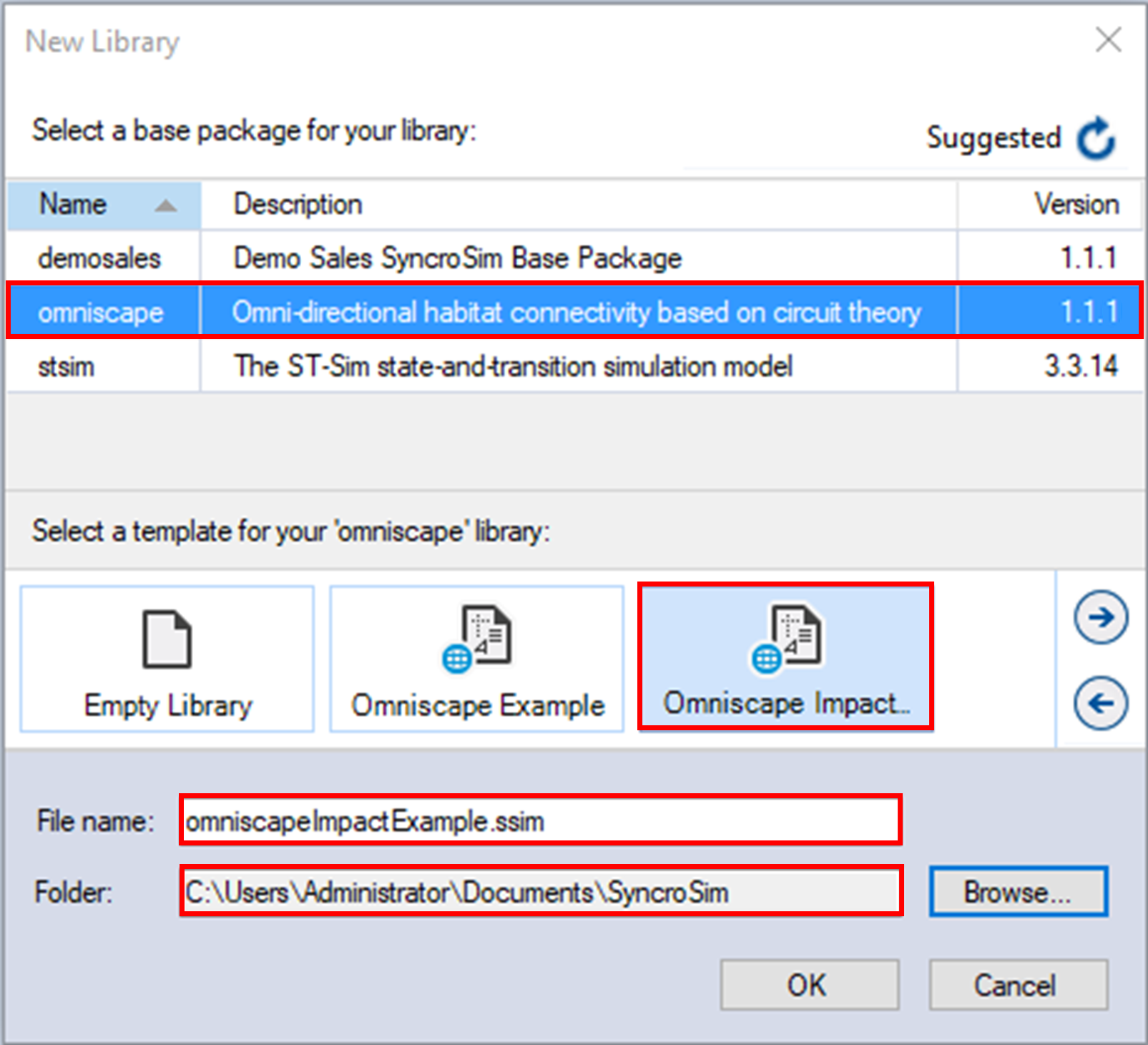
A new library will be created based on the selected template, and SyncroSim will automatically open and display it in the Library Explorer window.
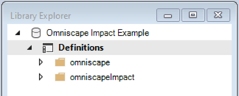
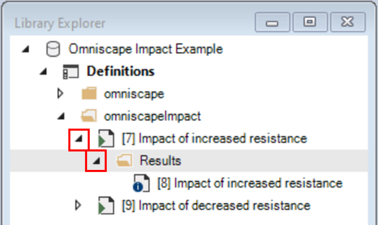
1. Note that the library contains two folders: omniscape and omniscapeImpact.
2. Expand the omniscape folder and note that it contains three scenarios.
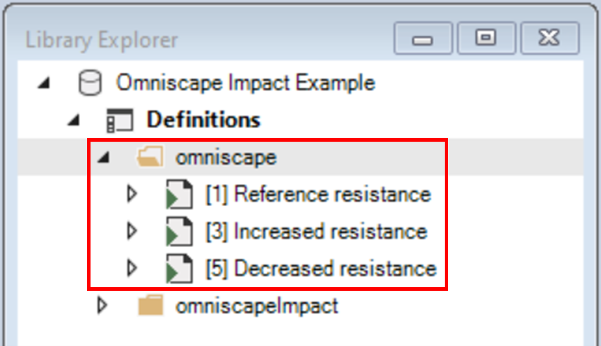
The additional scenario, Decreased resistance, represents the case where resistance has been decreased by a similar magnitude as in the Increased resistance scenario.
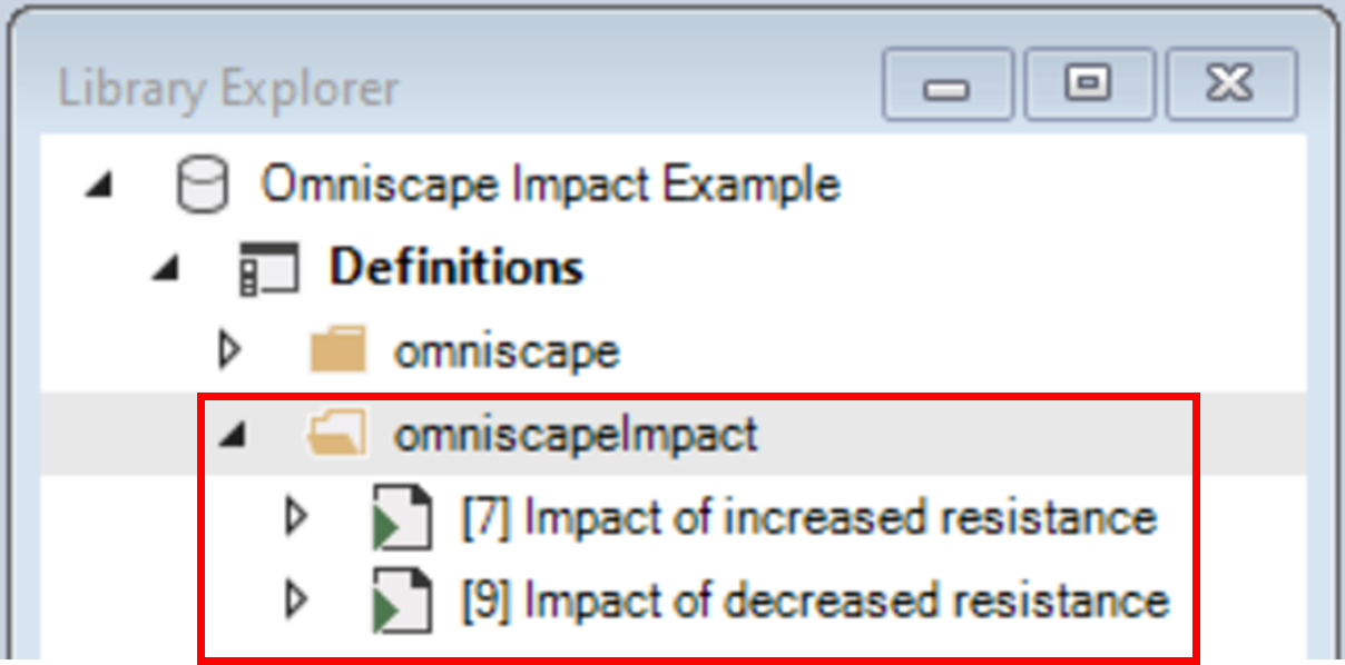
3. Next, expand the omniscapeImpact folder and note that it contains two scenarios:
b. Impact of decreased resistance – compares the Reference resistance and Decreased resistance scenarios.
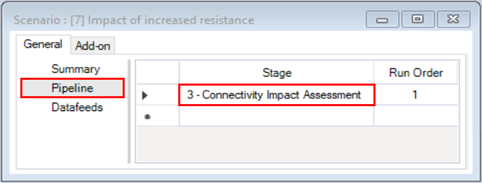
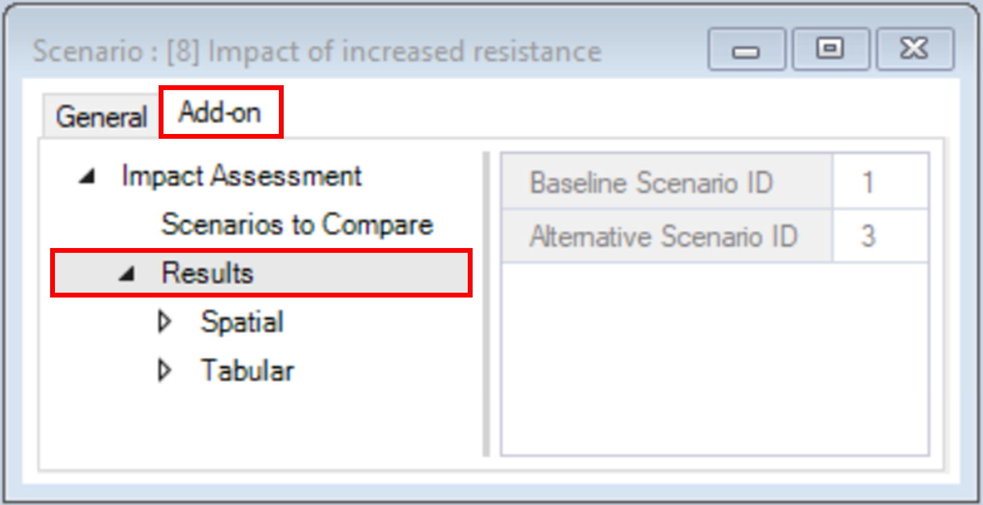
4. Double-click on Impact of increased resistance to open the scenario properties.
5. Under the General tab, navigate to the Pipeline datasheet.
6. Navigate to the Add-on tab.
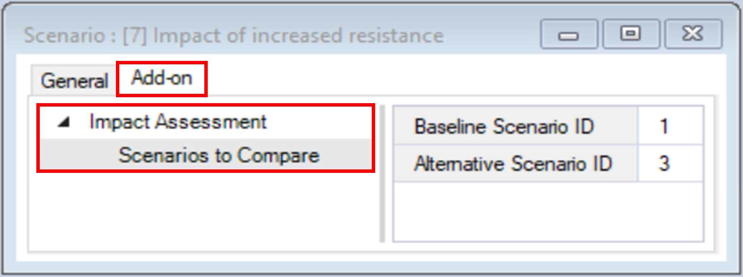
ii. Alternative Scenario ID – represents the changed connectivity state. For this example, the ID is 2 corresponding to the Increased resistance scenario.
7. Close the scenario properties.
Step 3. Visualizing and comparing scenario results
The Omniscape Impact template library already contains the results for all its scenarios. In SyncroSim, the results for a scenario are organized into a Results folder, nested within its parent scenario.
1. In the Library Explorer window, click on the arrow beside the Impact of increased resistance scenario to expose the Results folder; repeat the same action to expose the results scenario.
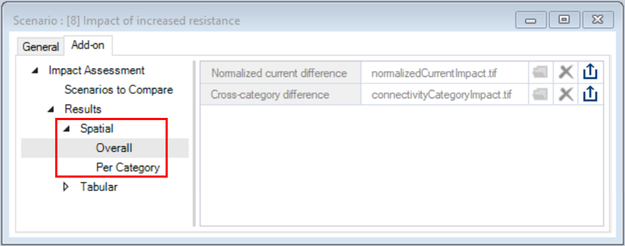
2. Double-click on the results scenario to open its properties.
3. Navigate to the Add-on tab and expand the Results node.
The omniscapeImpact package generates spatial and tabular outputs.
4. Under the Spatial node are the following outputs:
b. Per Category – represents per pixels loss, gain and no change for each connectivity category.
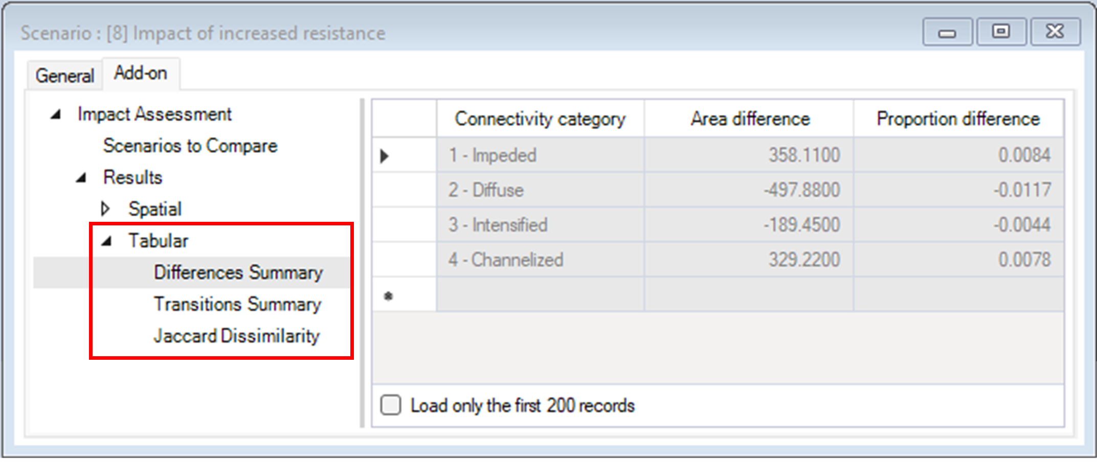
5. Under the Tabular node are the following outputs:
b. Transitions Summary – represents the change in area and proportion between the baseline and alternative scenarios for all possible transitions between connectivity categories.
c. Jaccard Dissimilarity – represents the dissimilarity between the baseline and alternative scenarios for each connectivity category. For each connectivity category, the Jaccard Dissimilarity is calculated as 1 minus the ratio between the number of shared pixels across scenarios and the total number of pixels across scenarios.
6. Close the scenario properties and collapse the results and scenario folder.
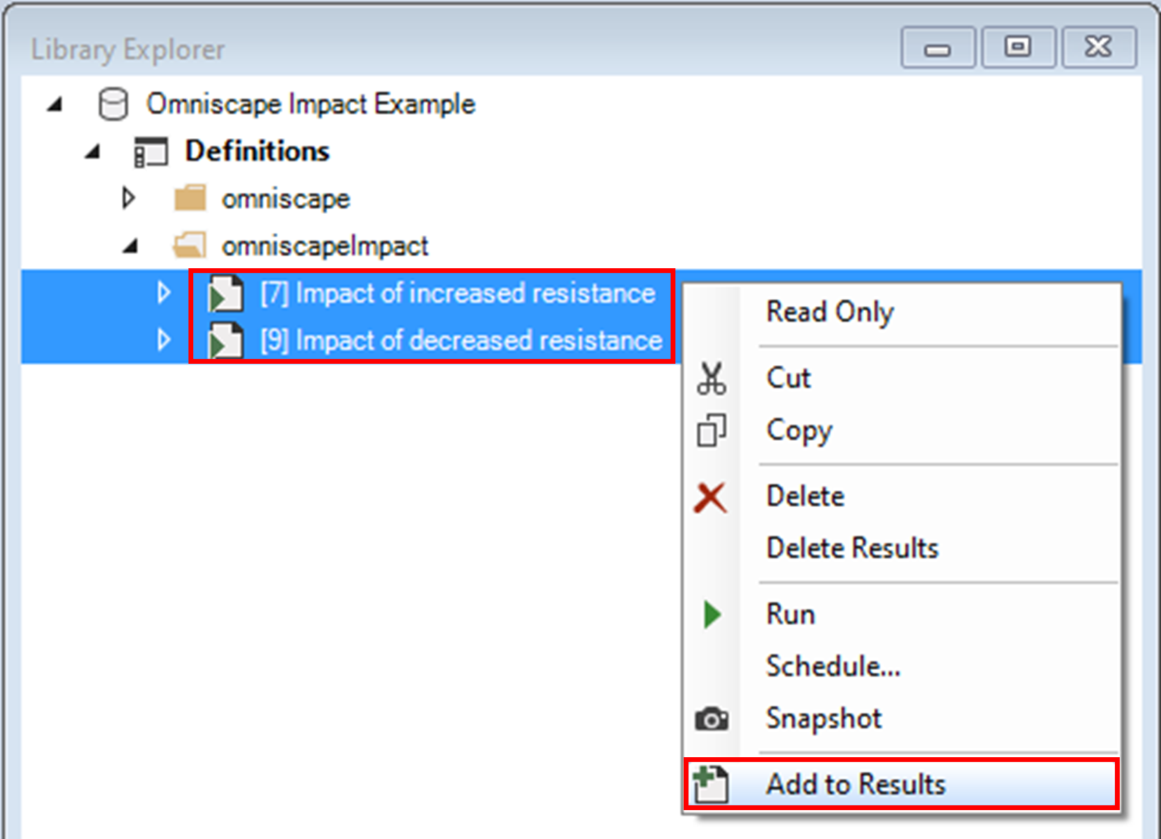
7. In the Library Explorer window, select the scenarios Impact of increased resistance and Impact of decreased resistance, right-click, and select Add to Results from the context menu.
8. Navigate to the Charts tab and double-click to view the Area difference chart.
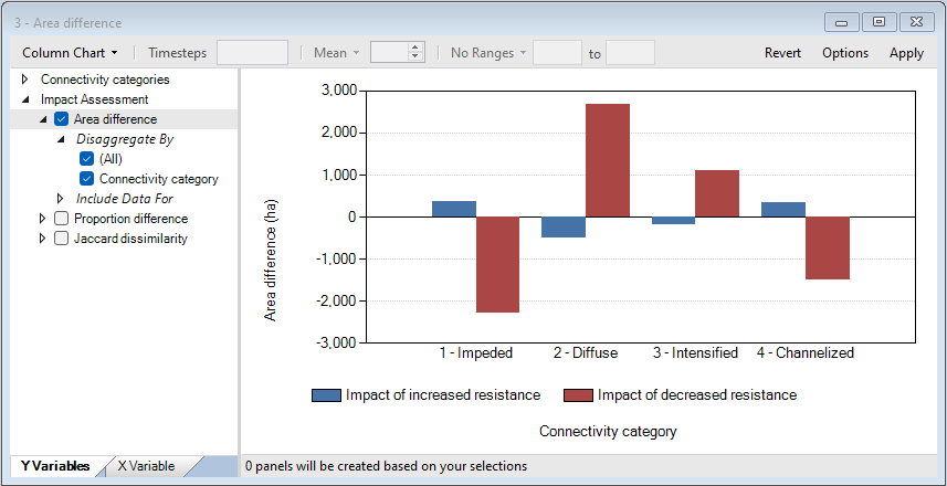
The Increased resistance scenario led to an increase in area for Impeded and Channelized and a decrease in area for Diffuse and Intensified, relative to the Reference scenario.
The Decreased resistance scenario led to a decrease in area for Impeded and Channelized and an increase in area for Diffuse and Intensified, relative to the Reference scenario.
Note also that the magnitude of change in area was larger under the Decreased resistance scenario.
9. Close the Area difference chart and open the Jaccard dissimilarity chart.
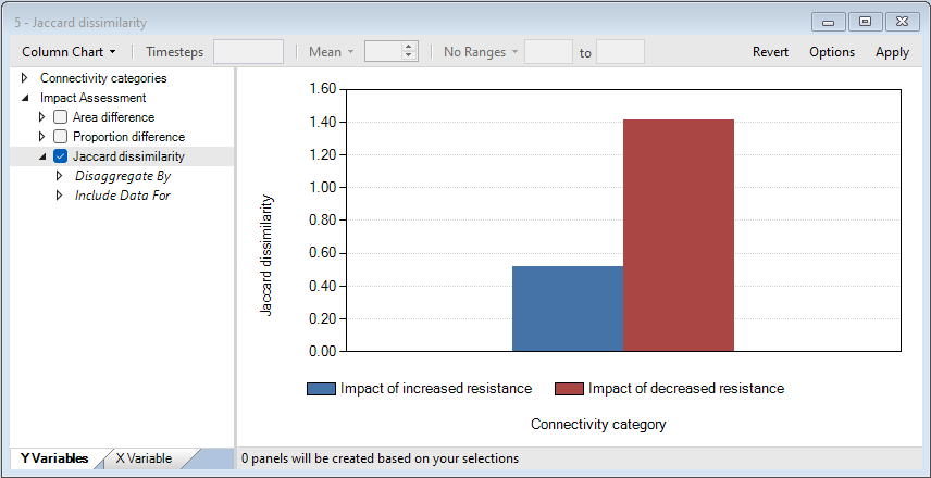
Next, for a visual confirmation of the quantitative changes summarized by area and the Jaccard dissimilarity, you will inspect the spatial outputs of omniscapeImpact.
10. Navigate to the Maps tab and double-click to open the Normalized current difference and Cross-category difference maps.
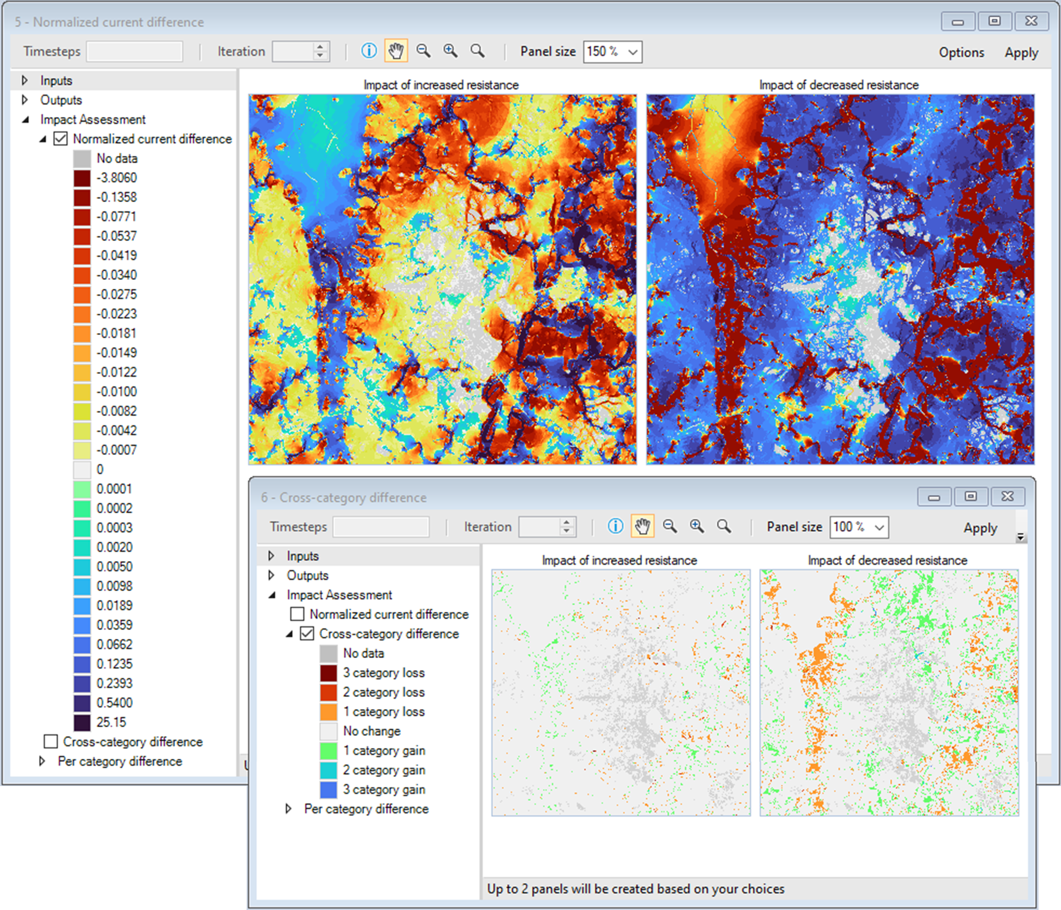
In turn, the Cross-category difference map highlights pixels where the change in current represented a change in connectivity category. For example, a change from Impeded to Diffuse would represent a 1 category gain, while a change from Channelized to Diffuse would represent a 2 category loss.
11. Close the Normalized current difference and open the Per-category difference map.

Both maps also highlight that a decrease in resistance had a stronger effect on connectivity than an increase.