Getting started with ST-Connect
Quickstart Tutorial
This quickstart tutorial will introduce you to the basics of working with ST-Connect. The steps include:
- Installing ST-Connect
- Creating a new ST-Connect Library
- Configuring the ST-Connect Library
- Viewing model inputs
- Running the model
- Analyzing the results
Step 1: Installing ST-Connect
ST-Connect is a Package within the SyncroSim simulation modeling framework. As such, running ST-Connect requires that the SyncroSim software be installed on your computer. Download the latest version of SyncroSim here.
ST-Connect also requires R version 4.0.4 or higher, and Circuitscape 5. If you wish to include Conservation Prioritization in your pipeline, download and install Zonation version 4.0.0.
Note: To download and install Circuitscape, follow the Circuitscape.jl installation link and not the link to the Windows executable. It will prompt you to install Julia first, which will then be used to install Circuitscape.
Once all required programs are installed, open SyncroSim and select File -> Packages… -> Install…, check the box for the stconnect package and click OK.
Step 2: Creating a new ST-Connect Library
Having installed the ST-Connect Package, you are now ready to create your first SyncroSim Library. A Library is a file (with extension .ssim) that contains all of your model inputs and outputs. To create a new Library, choose New Library… from the File menu.
- Select the row for stconnect - Connectivity planning for future climate and land-use change. Note that as you select a row, the list of Templates available and suggested File name for that base package are updated.
- Select the Simple Conn. Model Template.
- Type in a new File name for the Library or accept the default. You can also change the target Folder using the Browse… button.
Note: If you intend on using Multiprocessing (recommended), ensure your SyncroSim Library is saved to the C: Drive. Saving your library to OneDrive will result in an error when completing a model run.

When you are ready to create the Library file, click OK. A new Library will be created and loaded into the Library Explorer.
Step 3: Configuring the ST-Connect Library
For the model to run, SyncroSim needs to locate your R, Julia, and Zonation (if applicable) executables.
The R executable will be found automatically. To check, in the Library Explorer, double-click on hte Library Simple Conn. Model and navigate to the Options tab. In the R Configuration datasheet, you should see the file path to your R executable. If not, click Browse… and navigate to the correct file location.
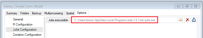
The default file location of the Julia executable is blank. Select the Folder icon, navigate to the proper location on your local computer (example shown below), then click Open.
Note: As shown below, the AppData folder will need to be accessed. This is normally a hidden folder on your computer. To access this folder, open your Windows Explorer, open the View tab, and enable Hidden Items.
Step 4: Viewing model inputs
The contents of your newly created Library are now displayed in the Library Explorer. Model inputs in SyncroSim are organized into Scenarios, where each Scenario consists of a suite of values, one for each of the model’s required inputs.
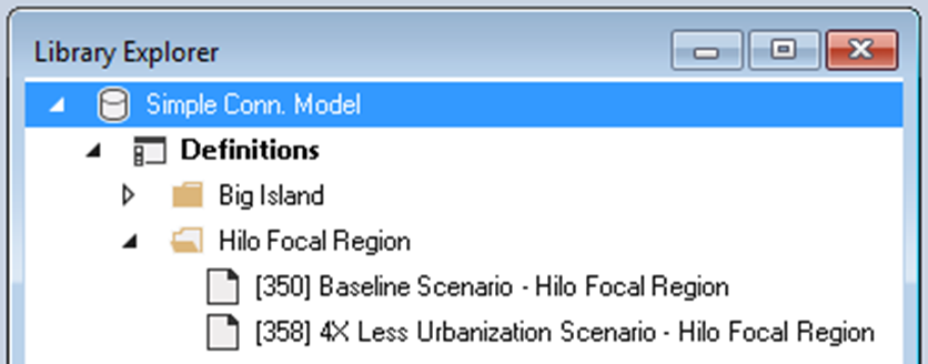
Because you chose the Simple Conn. Model Template when you created your Library, your Library already contains two Project folders (Big Island and Hilo Focal Region), each with two pre-configured Scenarios with model inputs derived from historical land change data. These inputs were filled in and distributed as a sample with the package to help you get started quickly, and represent hypothetical management scenarios. The Scenarios named 4X Less Urbanization Scenario contain model inputs corresponding to an alternative land management plan where urbanization targets are 4 times less than in the Baseline Scenario.
For the purposes of this Quickstart tutorial, you will run the Hilo Focal Region Project, with Scenarios IDs 350 and 358 (IDs shown below in square brackets). These Scenarios use cropped landscapes of the Big Island Scenarios and will take a significantly shorter amount of time to run. Explore the Big Island Scenarios afterwards if desired.
To view the details of the first of these Scenarios:
- Select the scenario named Baseline Scenario - Hilo Focal Region in the Library Explorer.
- Double-click, or right-click and choose Properties from the context menu to view the details of the Scenario.
This opens the Scenario Properties window:
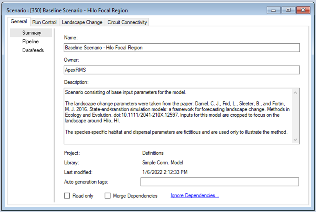
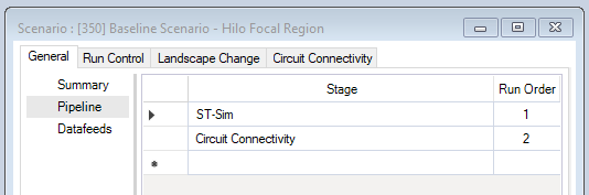
The first tab in this window, called General, contains three datasheets. The first, Summary, displays some general information for the Scenario. The second, Pipeline, allows the user to select the run order of the Stages in the pipeline.
Finally, the Datafeeds datasheet displays a list of all data sources input into the model.
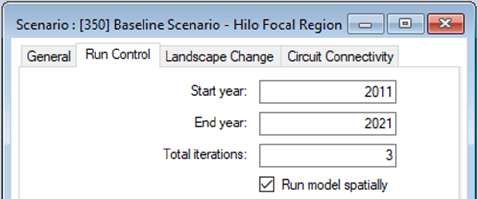
The second tab in the window, Run Control, contains parameters for running the model simulation. In this example, the Scenario will run for 10 years, starting in the year 2011, and is repeated for 3 Monte Carlo iterations.
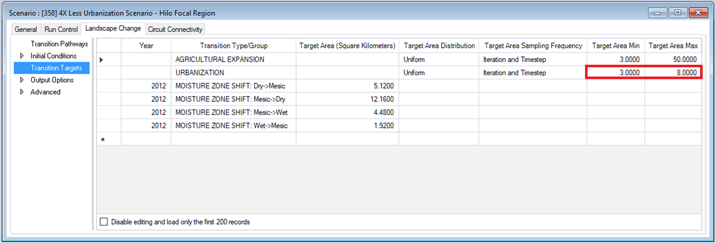
Click on the Landscape Change and Circuit Connectivity tabs to familiarize yourself with this Scenario’s inputs. In particular, under Landscape Change > Output Options > Output Options Spatial and Circuit Connectivity > Output Options, note that the output frequency is set to 10 years in order to speed up the run times and save on disk space. Also notice that, under Landscape Change > Transition Targets, the Baseline Scenario has a Urbanization target area of 12 to 32 sq. km.

Next, open the Scenario Properties window for the scenario named 4X Less Urbanization Scenario - Hilo Focal Region. Notice that the target minimum and maximum within the Urbanization transition type have decreased relative to the Baseline Scenario.
Step 5: Running the model
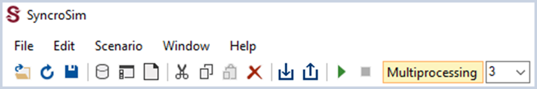
In the toolbar, enable Multiprocessing with 3 jobs. This will cut down the time required to run the simulation (~8 minutes when Multiprocessing is enabled, ~24 minutes when is disabled).
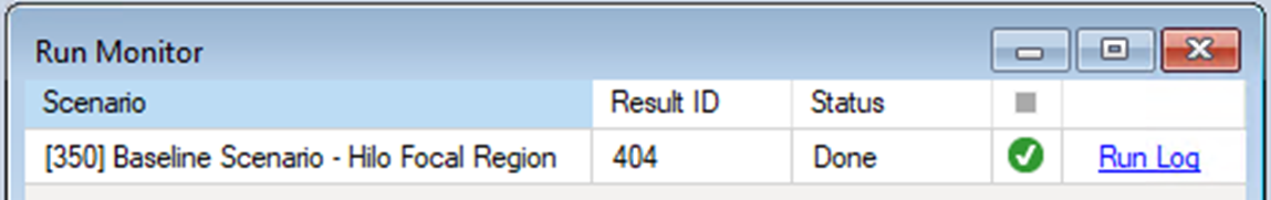
Right-click on the Baseline Scenario - Hilo Focal Region in the Scenario Manager window and select Run from the context menu. If prompted to save your project, click Yes. If the run is successful, you will see a Status of Done in the Run Monitor window, at which point you can close the Run Monitor window; otherwise, click on the Run Log link to see a report of any problems, make any necessary changes to your Scenario, then re-run the Scenario.
Run 4X Less Urbanization Scenario - Hilo Focal Region next by repeating the steps above.
Step 6: Analyzing the results
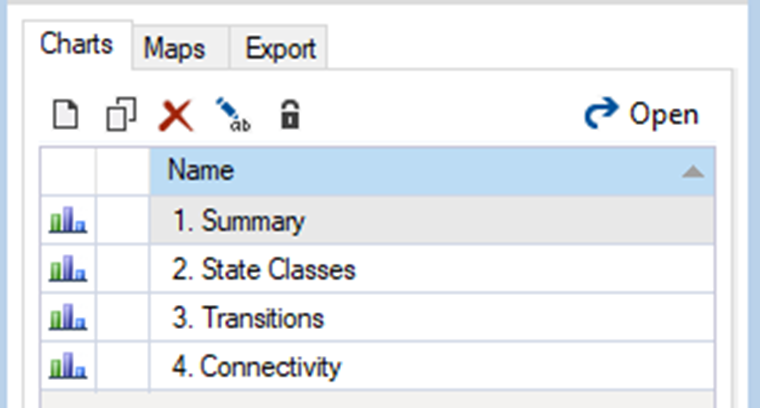
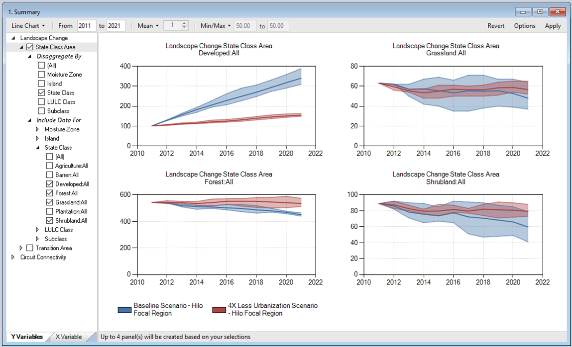
To view results from your run, move to the Charts tab at the bottom left of the Scenario Manager screen and double-click on Summary to open it.
You can now view and compare the results of running your two Scenarios through the model from the ST-Connect Package.
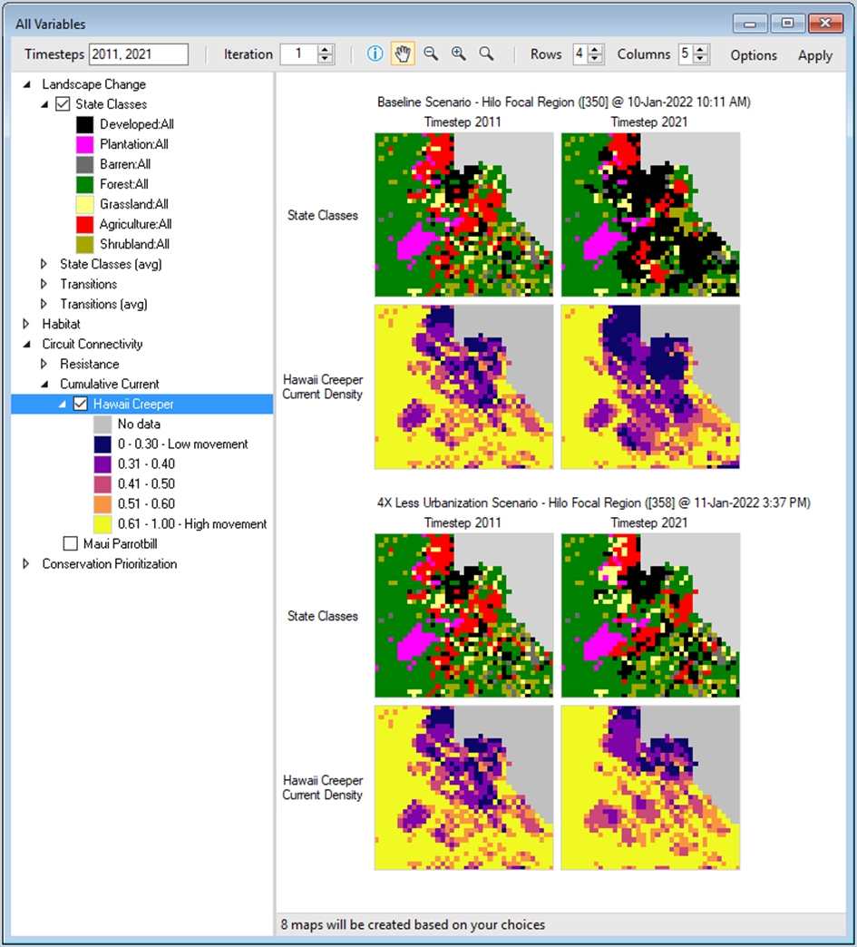
Next, select the Maps tab from the bottom of the Scenario Manager window (i.e., beside the Charts tab). Double click on All Variables. The mapping window should display changes in state class and circuit connectivity by default. In the state class maps, the Baseline Scenario results in a more drastic increase in developed land than the 4X Less Urbanization Scenario. As a consequence, the Baseline Scenario results in less movement across the landscape by 2021, compared to the 4X Less Urbanization Scenario.
Note: Legends can be customized by double-clicking on the bins.
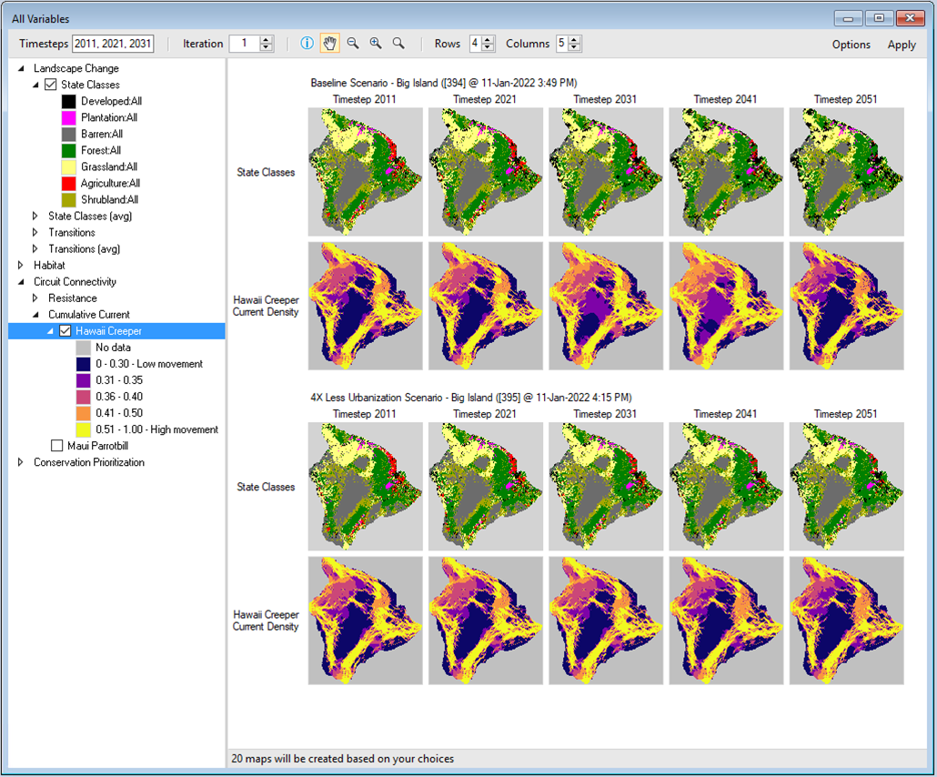
Scenarios featuring the entirety of Hawaii’s Big Island are included in the Library. Follow Steps 4 and 5 to explore these scenarios. Notice that these scenarios run from 2011 to 2051. Expect the model run to take about 1.5 hours per scenario.
Note: You can add and remove Results Scenarios from the list of scenarios being analyzed by selecting a Scenario in the Library Explorer and then choosing either Add to Results or Remove from Results from the Scenario menu. Scenarios currently selected for analysis are highlighted in bold in the Library Explorer. When adding or removing results from the Scenario menu, make sure to click on “Full Zoom”, in the mapping window, after the desired scenarios are selected.
Learn more
- For an example of an application of ST-Connect, see this study.
- For more on Circuitscape, see the Circuitscape documentation.
- For more on connectivity forecasting research, see the special issue Dynamic Landscape Connectivity.